Distances and Time Series

We will start building some tools for making comparisons of data objects with particular attention to time series.

Working with data, we can encounter a wide variety of different data objects

  • records of users,
  • images,
  • videos,
  • text (webpages, books),
  • strings (DNA sequences), and
  • time series.

How can we compare them?

Lecture Overview

We cover the following topics in today’s lecture

  • feature space and matrix representations of data,
  • metrics, norms, similarity, and dissimilarity,
  • bit vectors, sets, and time series.

Time Series Data

Some examples of time series data

  • stock prices,
  • weather data,
  • electricity consumption,
  • website traffic,
  • retail sales, and
  • various economic indicators.

Feature space representation

Usually a data object consists of a set of attributes.

These are also commonly called features.

  • (“J. Smith”, 25, $ 200,000)
  • (“M. Jones”, 47, $ 45,000)

If all \(d\) dimensions are real-valued then we can visualize each data object as a point in a \(d\)-dimensional vector space.

  • (25, USD 200000) \(\rightarrow \begin{bmatrix}25\\200000\end{bmatrix}\).

Likewise If all features are binary then we can think of each data object as a binary vector in vector space.

The space is called feature space.

One-hot encoding

Vector spaces are such a useful tool that we often use them even for non-numeric data.

For example, consider a categorical variable that can be only one of “house”, “tree”, or “moon”. For such a variable, we can use a one-hot encoding.

  • house: \([1, 0, 0]\)
  • tree: \([0, 1, 0]\)
  • moon: \([0, 0, 1]\)

So an encoding of (25, USD 200000, 'house') could be: \[\begin{bmatrix}25\\200000\\1\\0\\0\end{bmatrix}.\]

Why not alternative encoding?

Why would we not encode as follows:

  • house: \([1]\)
  • tree: \([2]\)
  • moon: \([3]\)

So an encoding of (25, USD 200000, 'house') could be: \[\begin{bmatrix}25\\200000\\1\end{bmatrix}.\]

This is not a good idea because it implicitly assumes that the categories are ordered.

One hot encoding treats the categorical data as orthogonal from a vector space perspective.

🎯 Class Activity: Feature Encoding

Task: Work in pairs to encode the following data into feature vectors.

Data to encode:

  • Person A: (age=30, salary=$75,000, city=“New York”, education=“PhD”)
  • Person B: (age=25, salary=$50,000, city=“Boston”, education=“Masters”)
  • Person C: (age=35, salary=$90,000, city=“New York”, education=“Bachelors”)

Instructions:

  1. Create one-hot encodings for categorical variables (city: NY, Boston, LA; education: Bachelors, Masters, PhD)
  2. Normalize the numerical features (age: divide by 100, salary: divide by 100,000)
  3. Write out the complete feature vectors for all three people
  4. Calculate the Euclidean distance between Person A and Person B

Discussion: Why might we normalize numerical features? What does the distance tell us about similarity?

Encodings

We will see many other encodings that take non-numeric data and encode them into vectors or matrices.

For example, there are vector or matrix encodings for

  • graphs,
  • images, and
  • text.

Matrix representation of data

We generally store data in a matrix form as

\[ \mbox{$m$ data objects}\left\{\begin{array}{c}\;\\\;\\\;\\\;\\\;\end{array}\right.\;\;\overbrace{\left[\begin{array}{ccccc} \begin{array}{c} x_{11} \\ \vdots \\ x_{i1} \\ \vdots \\ x_{m1} \end{array}& \begin{array}{c} \cdots \\ \ddots \\ \cdots \\ \ddots \\ \cdots \end{array}& \begin{array}{c} x_{1j} \\ \vdots \\ x_{ij} \\ \vdots \\ x_{mj} \end{array}& \begin{array}{c} \cdots \\ \ddots \\ \cdots \\ \ddots \\ \cdots \end{array}& \begin{array}{c} x_{1n} \\ \vdots \\ x_{in} \\ \vdots \\ x_{mn} \end{array} \end{array}\right]}^{\mbox{$n$ features}} \]

The number of rows is denoted by \(m\) and the number of columns by \(n\). The rows are instances or records of data and the columns are the features.

Metrics

A metric is a function \(d(x, y)\) that satisfies the following properties.

  • \(d(x, x) = 0\)
  • \(d(x, y) > 0 \hspace{1cm} \forall x\neq y\) (positivity)
  • \(d(x, y) = d(y, x)\) (symmetry)
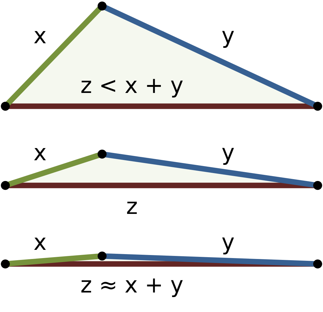
  • \(d(x, y)\leq d(x, z) + d(z, y)\) (triangle inequality)

We can use a metric to determine how similar or dissimilar two objects are.

A metric is a measure of the dissimilarity between two objects. The larger the measure, the more dissimilar the objects are.

If the objects are vectors, then the metric is also commonly called a distance.

Distance Matrices

The distance matrix is defined as

\[ \mbox{$m$ data objects}\left\{\begin{array}{c}\;\\\;\\\;\\\;\\\;\end{array}\right.\;\; \overbrace{\left[\begin{array}{ccccc} \begin{array}{c} 0 \\ d(x_1, x_2) \\ d(x_1,x_3) \\ \vdots \\ d(x_1,x_m) \end{array} & \begin{array}{c} \; \\ 0 \\ d(x_2,x_3) \\ \vdots \\ d(x_2,x_m) \end{array} & \begin{array}{c} \; \\ \; \\ 0 \\ \vdots \\ \cdots \end{array} & \begin{array}{c} \; \\ \; \\ \; \\ \ddots \\ d(x_{m-1},x_m) \end{array} & \begin{array}{c} \; \\ \; \\ \; \\ \; \\[6pt] 0 \end{array} & \end{array}\right]}^{\mbox{$m$ data objects}}, \]

where \(x_i\) denotes the \(i\)-th row of the data matrix \(X\).

Norms

Let \(\mathbf{u}, \mathbf{v}\in\mathbb{R}^{n}\) and \(a\in\mathbb{R}\). The vector function \(p(\mathbf{v})\) is called a norm if

  • \(p(a\mathbf{v}) = |a|p(\mathbf{v})\),
  • \(p(\mathbf{u} + \mathbf{v}) \leq p(\mathbf{u}) + p(\mathbf{v})\),
  • \(p(\mathbf{v}) = 0\) if and only if \(\mathbf{v} = 0\).

Every norm defines a corresponding metric.

In particular If \(p()\) is a norm, then \(d(\mathbf{x}, \mathbf{y}) = p(\mathbf{x}-\mathbf{y})\) is a metric.

But not every metric can be derived from a norm!

For example, the discrete metric is not a norm. \[ d(x,y) = \begin{cases} 0 & x=y \\ 1 & x \neq y \end{cases} \]

\(\ell_p\) norm

A general class of norms are called \(\ell_p\) norms, where \(p \geq 1.\)

\[ \Vert \mathbf{x} \Vert_p = \left(\sum_{i=1}^d |x_i|^p\right)^{\frac{1}{p}}. \]

The corresponding distance that an \(\ell_p\) norm defines is called the Minkowski distance.

\[ \Vert \mathbf{x} - \mathbf{y} \Vert_p = \left(\sum_{i=1}^d |x_i - y_i|^p\right)^{\frac{1}{p}}. \]

The choice of \(p\) affects what gets emphasized in the distance calculation:

  • For small \(p\) (e.g. \(p=1\)):
    • More emphasis on many small differences
    • Less sensitive to outliers/large differences
  • For large \(p\) (e.g. \(p\rightarrow \infty\)):
    • More emphasis on the largest difference
    • Very sensitive to outliers

\(\ell_2\) norm

A special – but very important – case is the \(\ell_2\) norm.

\[ \Vert \mathbf{x} \Vert_2 = \sqrt{\sum_{i=1}^d |x_i|^2}. \]

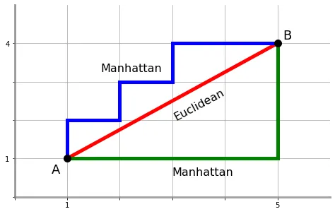
We’ve already mentioned it: it is the Euclidean norm.

The distance defined by the \(\ell_2\) norm is the same as the Euclidean distance between two vectors \(\mathbf{x}, \mathbf{y}\).

\[ \Vert \mathbf{x} - \mathbf{y} \Vert_2 = \sqrt{\sum_{i=1}^d (x_i - y_i)^2}. \]

\(\ell_1\) norm

Another important special case is the \(\ell_1\) norm.

\[ \Vert \mathbf{x} \Vert_1 = \sum_{i=1}^d |x_i|.\]

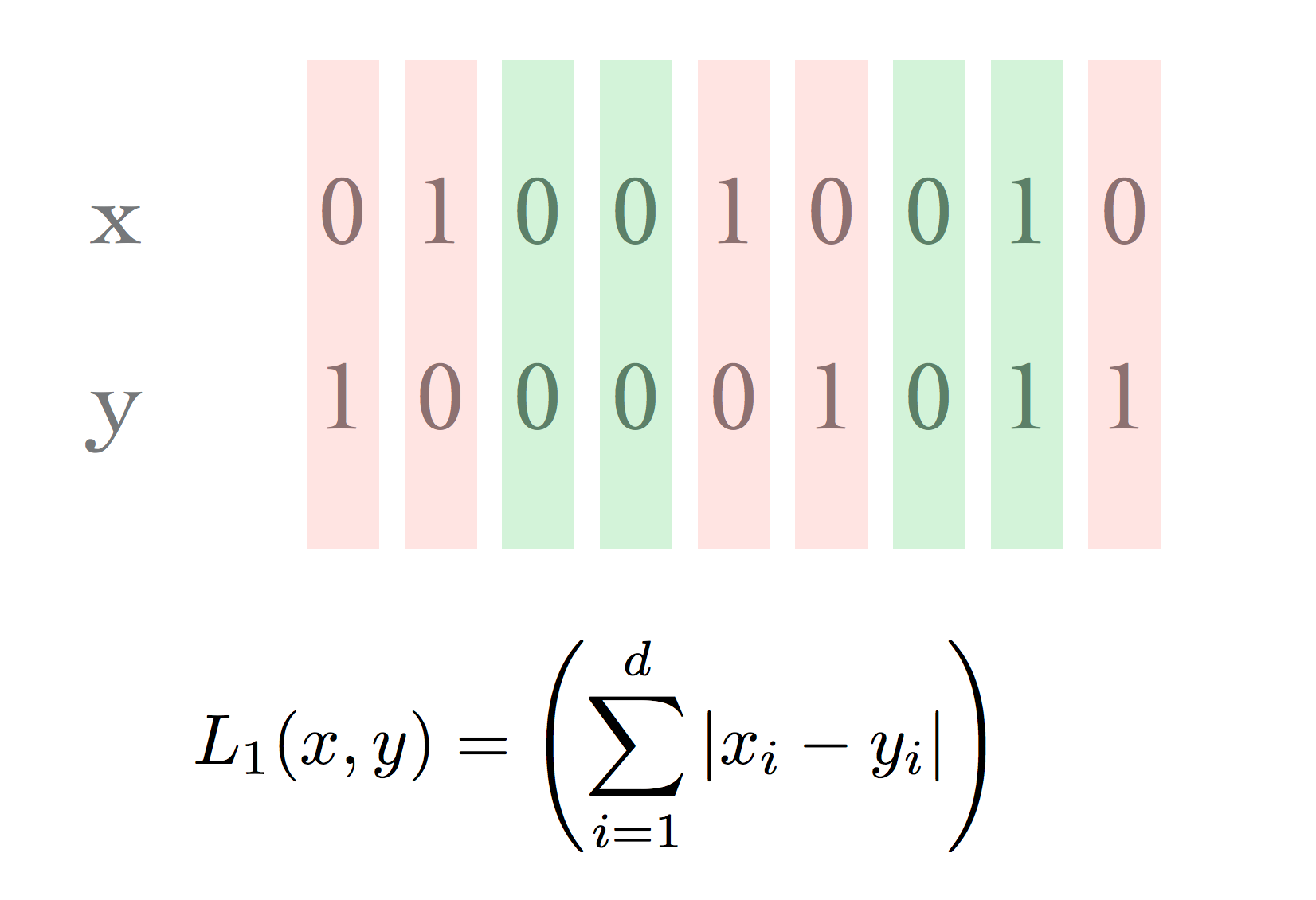
This defines the Manhattan distance, or (for binary vectors), the Hamming distance:

\[ \Vert \mathbf{x} - \mathbf{y} \Vert_1 = \sum_{i=1} |x_i - y_i|.\]

\(\ell_\infty\) norm

If we take the limit of the \(\ell_p\) norm as \(p\) gets large we get the \(\ell_\infty\) norm.

We have that

\[ \Vert \mathbf{x} \Vert_{\infty} = \max_{i} \vert x_{i} \vert . \]

What is the metric that this norm induces?

Answer: The \(\ell_\infty\) norm induces the Chebyshev distance which is also known as the maximum distance.

\[ \Vert \mathbf{x} - \mathbf{y} \Vert_{\infty} = \max_{i} \vert x_{i} - y_{i} \vert . \]

Visualizing norms

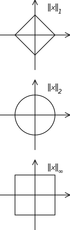
Here is the notion of a “circle” under each of three norms.

That is, for each norm, the set of vectors having norm 1, or distance 1 from the origin.


\(|x_1| + |x_2| = 1\)


\(\sqrt{x_1^2 + x_2^2} = 1\)


\(\max(|x_1|, |x_2|) = 1\)

Source

What norm should I use?

The choice of norm depends on the characteristics of your data and the problem you’re trying to solve.

\(\ell_1\) norm

  • Use when your data is sparse.
  • Robust to outliers.

\(\ell_2\) norm

  • Use when measuring distances in Euclidean space.
  • Smooth and differentiable.

\(\ell_\infty\) norm

  • Use when you need uniform bounds.
  • Limits maximum deviation.

🎯 Class Activity: Norm Comparison

Task: Compare how different norms measure distance between the same two points.

Given: Two 2D points A = (3, 4) and B = (1, 1)

Instructions:

  1. Calculate the distance between A and B using:
    • \(\ell_1\) norm (Manhattan distance)
    • \(\ell_2\) norm (Euclidean distance)
    • \(\ell_\infty\) norm (Chebyshev distance)
  2. Now consider points C = (0, 0) and D = (1, 0)
    • Calculate all three distances again
    • Which norm gives the smallest distance? Largest?
  3. Think-pair-share:
    • In what real-world scenarios would you prefer each norm?
    • How does the choice of norm affect outlier sensitivity?

Bonus: Sketch the “unit circles” for each norm in 2D space.

Similarity and Dissimilarity Functions

Similarity functions quantify how similar two objects are. The higher the similarity score, the more alike the objects.

Examples

  • cosine similarity,
  • Jaccard similarity (intersection over union).

Dissimilarity functions quantifies the difference between two objects. The higher the dissimilarity score, the more different the objects are.

Examples

  • Manhattan distance,
  • Hamming distance.

Similarity

We know that the inner product of two vectors can be used to compute the cosine of the angle between them

\[ \cos(\theta) = \frac{\mathbf{x}^T\mathbf{y}}{\Vert\mathbf{x}\Vert \Vert\mathbf{y}\Vert} \equiv \cos(\mathbf{x}, \mathbf{y}) .\]

This value is

  • close to 1 when \(\mathbf{x} \approx \mathbf{y}\) (\(\theta \approx 0\)) and
  • close to 0 when \(\mathbf{x}\) and \(\mathbf{y}\) are orthogonal (\(\theta \approx 90^\circ\)).

We can use this formula to define a similarity function called the cosine similarity \(\cos(\mathbf{x}, \mathbf{y})\).


Abuse of notation? 🤔

Dissimilarity

Given a similarity function \(s(\mathbf{x}, \mathbf{y})\), how could we convert it to a dissimilarity function \(d(\mathbf{x}, \mathbf{y})\)?

Two straightforward ways of doing that are:

\[d(\mathbf{x},\mathbf{y}) = 1\,/\,s(\mathbf{x},\mathbf{y})\]

or

\[d(\mathbf{x},\mathbf{y}) = k - s(\mathbf{x},\mathbf{y})\]

for some properly chosen \(k\).

For cosine similarity, one often uses:

\[ d(\mathbf{x}, \mathbf{y}) = 1 - \cos(\mathbf{x}, \mathbf{y})\]

🎯 Class Activity: Similarity Calculations

Task: Calculate different similarity measures between two documents represented as word frequency vectors.

Given: Two documents with word counts:

  • Document A: [cat: 3, dog: 2, bird: 1, fish: 0]
  • Document B: [cat: 1, dog: 3, bird: 0, fish: 2]

Instructions:

  1. Convert to normalized vectors (divide by total word count)
  2. Calculate cosine similarity between the documents
  3. Calculate the dissimilarity using: d = 1 - cosine_similarity
  4. Quick discussion:
    • What does a cosine similarity of 0.5 mean?
    • Why might cosine similarity be better than Euclidean distance for text documents?

Solution

Code
import numpy as np
from sklearn.metrics.pairwise import cosine_similarity

def calculate_document_similarity():
    """
    Calculate different similarity measures between two documents represented as word frequency vectors.
    """
    print("Document Similarity Analysis")
    print("=" * 40)
    
    # Given word frequency vectors
    doc_a = np.array([3, 2, 1, 0])  # [cat, dog, bird, fish]
    doc_b = np.array([1, 3, 0, 2])  # [cat, dog, bird, fish]
    
    print("Original word frequency vectors:")
    print(f"Document A: {doc_a} (cat: 3, dog: 2, bird: 1, fish: 0)")
    print(f"Document B: {doc_b} (cat: 1, dog: 3, bird: 0, fish: 2)")
    print()
    
    # Step 1: Convert to normalized vectors (divide by total word count)
    doc_a_normalized = doc_a / np.sum(doc_a)
    doc_b_normalized = doc_b / np.sum(doc_b)
    
    print("Step 1: Normalized vectors (divided by total word count)")
    print(f"Document A normalized: {doc_a_normalized}")
    print(f"Document B normalized: {doc_b_normalized}")
    print(f"Sum of normalized A: {np.sum(doc_a_normalized):.6f}")
    print(f"Sum of normalized B: {np.sum(doc_b_normalized):.6f}")
    print()
    
    # Step 2: Calculate cosine similarity
    # Reshape for sklearn's cosine_similarity function
    doc_a_reshaped = doc_a_normalized.reshape(1, -1)
    doc_b_reshaped = doc_b_normalized.reshape(1, -1)
    
    cosine_sim = cosine_similarity(doc_a_reshaped, doc_b_reshaped)[0][0]
    
    print("Step 2: Cosine similarity calculation")
    print(f"Cosine similarity: {cosine_sim:.6f}")
    print()
    
    # Manual calculation for verification
    dot_product = np.dot(doc_a_normalized, doc_b_normalized)
    norm_a = np.linalg.norm(doc_a_normalized)
    norm_b = np.linalg.norm(doc_b_normalized)
    cosine_sim_manual = dot_product / (norm_a * norm_b)
    
    print("Manual verification:")
    print(f"Dot product: {dot_product:.6f}")
    print(f"Norm of A: {norm_a:.6f}")
    print(f"Norm of B: {norm_b:.6f}")
    print(f"Cosine similarity (manual): {cosine_sim_manual:.6f}")
    print()
    
    # Step 3: Calculate dissimilarity
    dissimilarity = 1 - cosine_sim
    
    print("Step 3: Dissimilarity calculation")
    print(f"Dissimilarity (1 - cosine_similarity): {dissimilarity:.6f}")
    print()
    
    # Additional analysis
    print("Additional Analysis:")
    print("-" * 20)
    
    # Euclidean distance for comparison
    euclidean_dist = np.linalg.norm(doc_a_normalized - doc_b_normalized)
    print(f"Euclidean distance: {euclidean_dist:.6f}")
    
    # Manhattan distance
    manhattan_dist = np.sum(np.abs(doc_a_normalized - doc_b_normalized))
    print(f"Manhattan distance: {manhattan_dist:.6f}")
    print()
    
    return {
        'doc_a_normalized': doc_a_normalized,
        'doc_b_normalized': doc_b_normalized,
        'cosine_similarity': cosine_sim,
        'dissimilarity': dissimilarity,
        'euclidean_distance': euclidean_dist,
        'manhattan_distance': manhattan_dist
    }

if __name__ == "__main__":
    results = calculate_document_similarity()
Document Similarity Analysis
========================================
Original word frequency vectors:
Document A: [3 2 1 0] (cat: 3, dog: 2, bird: 1, fish: 0)
Document B: [1 3 0 2] (cat: 1, dog: 3, bird: 0, fish: 2)

Step 1: Normalized vectors (divided by total word count)
Document A normalized: [0.5        0.33333333 0.16666667 0.        ]
Document B normalized: [0.16666667 0.5        0.         0.33333333]
Sum of normalized A: 1.000000
Sum of normalized B: 1.000000

Step 2: Cosine similarity calculation
Cosine similarity: 0.642857

Manual verification:
Dot product: 0.250000
Norm of A: 0.623610
Norm of B: 0.623610
Cosine similarity (manual): 0.642857

Step 3: Dissimilarity calculation
Dissimilarity (1 - cosine_similarity): 0.357143

Additional Analysis:
--------------------
Euclidean distance: 0.527046
Manhattan distance: 1.000000

Discussion points

  1. What does a cosine similarity of 0.5 mean?

A cosine similarity of 0.5 means the documents are moderately similar. The angle between their vectors is approximately 60 degrees. This indicates some overlap in word usage patterns but not complete similarity.

  1. Why might cosine similarity be better than Euclidean distance for text documents?

Scale invariance: Cosine similarity focuses on the direction of vectors, not their magnitude, so document length doesn’t affect the comparison.

Normalization: It naturally handles documents of different lengths. Word frequency interpretation: It measures the relative proportion of words, which is more meaningful for text analysis than absolute differences.

Range: Cosine similarity ranges from -1 to 1, with 1 being identical, making it more interpretable for similarity measures.

Bit vectors and Sets

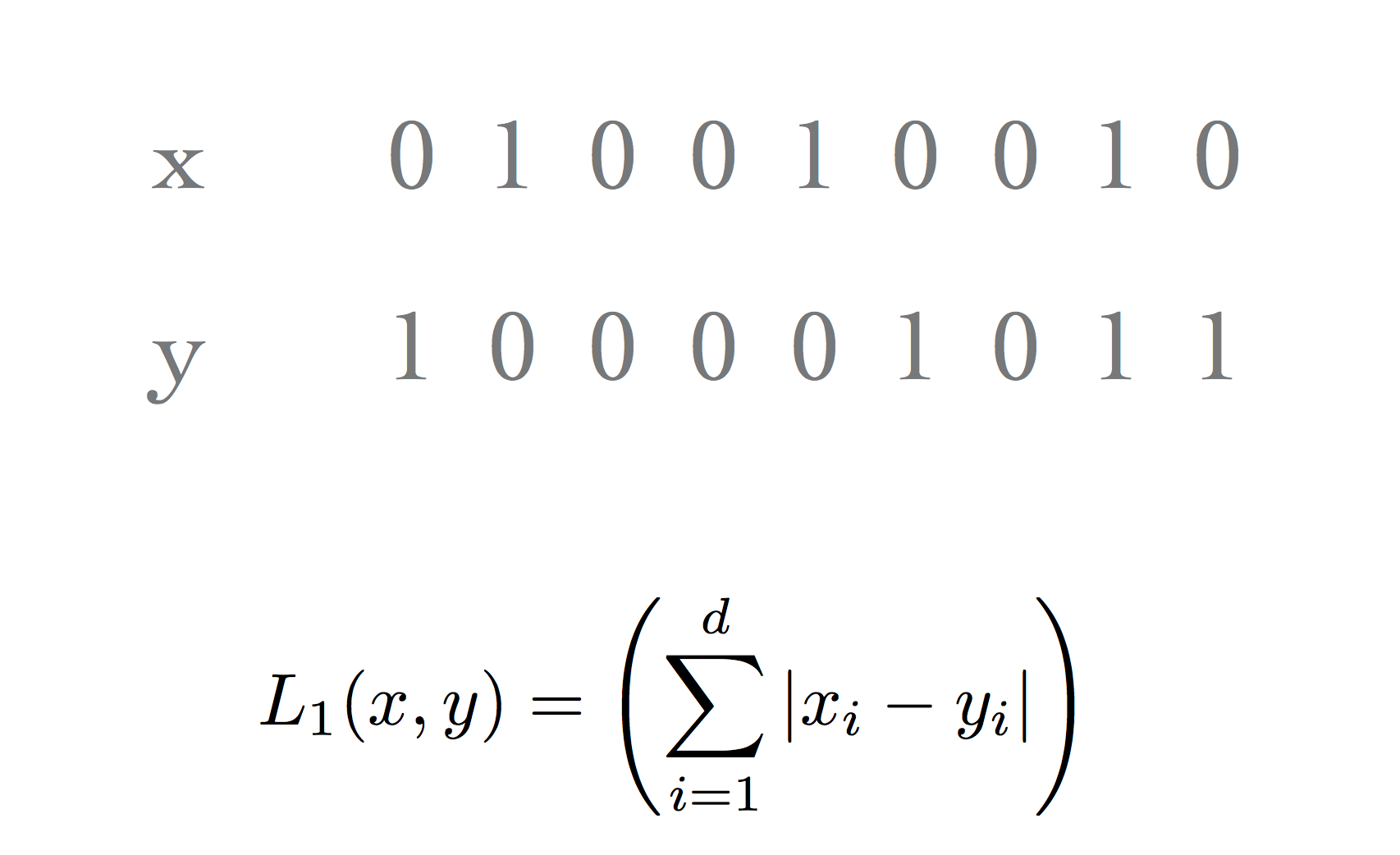
When working with bit vectors, the \(\ell_1\) metric is commonly used and is called the Hamming distance.

This has a natural interpretation: “how well do the two vectors match?”

Or: “What is the smallest number of bit flips that will convert one vector into the other?”

Hamming distance

Hamming distance with sets

Consider the case in which the bit vector is being used to represent a set.

Definition: A set is an unordered collection of distinct elements.

In that case, Hamming distance measures the size of the set difference.

For example, consider two documents. We will use bit vectors to represent the sets of words in each document.

  • Case 1: both documents are large, almost identical, but differ in 10 words.
  • Case 2: both documents are small, disjoint, have 5 words each.

What is the Hamming distance for each case?

\(L_1(\text{Case 1}) = 10\) and \(L_1(\text{Case 2}) = 5\). Is case 1 really more different than case 2?

What matters is not just the size of the set difference, but the size of the normalized intersection.

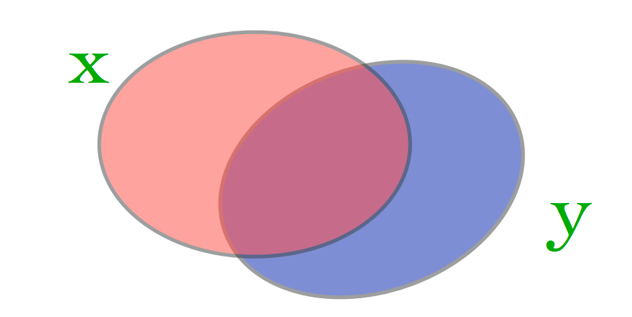
Jaccard similarity

This leads to the Jaccard similarity or Intersection over Union (IoU):

\[ J_{Sim}(\mathbf{x}, \mathbf{y}) = \frac{|\mathbf{x} \cap \mathbf{y}|}{|\mathbf{x} \cup \mathbf{y}|}. \]

This takes on values from 0 to 1, so a natural dissimilarity metric is \(1 - J_{Sim}().\)

In fact, this is a metric!

\[ J_{Dist}(\mathbf{x}, \mathbf{y}) = 1- \frac{|\mathbf{x} \cap \mathbf{y}|}{|\mathbf{x} \cup \mathbf{y}|}. \]

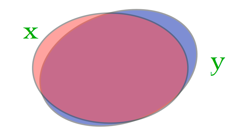
Jaccard Similarity Example 1

Case 1: Very large almost identical documents.

Here \(J_{Sim}(\mathbf{x}, \mathbf{y})\) is almost 1.

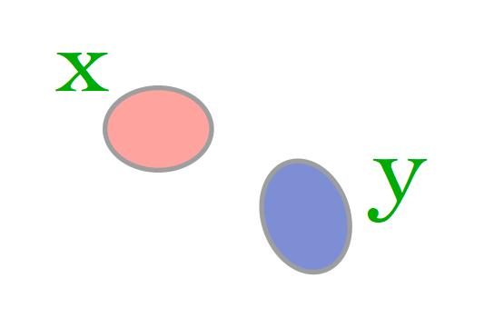
Jaccard Similarity Example 2

Case 2: Very small disjoint documents.

Here \(J_{Sim}(\mathbf{x}, \mathbf{y})\) is 0.

🎯 Class Activity: Jaccard Similarity Practice

Task: Calculate Jaccard similarity for different document scenarios.

Given: Three documents represented as sets of unique words:

  • Document 1: {apple, banana, cherry, date}
  • Document 2: {apple, banana, cherry, elderberry}
  • Document 3: {grape, kiwi, lemon, mango}

Instructions:

  1. Calculate Jaccard similarity between:
    • Document 1 and Document 2
    • Document 1 and Document 3
    • Document 2 and Document 3
  2. Think-pair-share:
    • Which pair is most similar? Least similar?
    • How does this compare to what you’d expect from Hamming distance?
    • When would you prefer Jaccard similarity over Hamming distance?

Real-world application: Consider how this applies to comparing user preferences, shopping baskets, or social media interests.

Time Series

A time series is a sequence of real numbers, representing the measurements of a real variable at (possibly equal) time intervals.

Some examples are

  • stock prices,
  • the volume of sales over time, and
  • daily temperature readings.

A time series database is a large collection of time series.

Similarity of Time Series

Suppose we wish to compare the following time series.

  • Stock price movements for companies over a time interval.
  • The motion data of two people walking.
  • Credit usage patterns for bank clients.

How should we measure the “similarity” of these time series?

There are two problems to address.

  1. Defining a meaningful similarity (or distance) function.
  2. Finding an efficient algorithm to compute it.

Norm-based Similarity Measures

We could just view each sequence as a vector.

Then we could use a \(p\)-norm, e.g., \(\ell_1, \ell_2,\) or \(\ell_p\) to measure similarity.

Advantages

  1. Easy to compute - linear in the length of the time series (O(n)).
  2. It is a metric.

Beware of Norm-based Similarity

Disadvantage

  1. May not be meaningful!

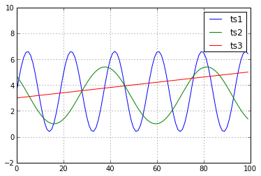
We may believe that \(\mathbf{ts1}\) and \(\mathbf{ts2}\) are the most “similar” pair of time series.

However, according to Euclidean distance:

\[ \Vert \mathbf{ts1} - \mathbf{ts2} \Vert_2 = 26.9,\]

while

\[ \Vert \mathbf{ts1} - \mathbf{ts3} \Vert_2 = 23.2.\]

Feature Engineering

Feature engineering is the art of computing some derived measure from your data object that makes the important properties usable in a subsequent step.

A reasonable approach is to

  • extract the relevant features,
  • use a simple method (e.g., a norm) to define similarity over those features.

In the case above, one might think of using

  • Fourier coefficients (to capture periodicity),
  • histograms,
  • or something else!

Bump Hunting

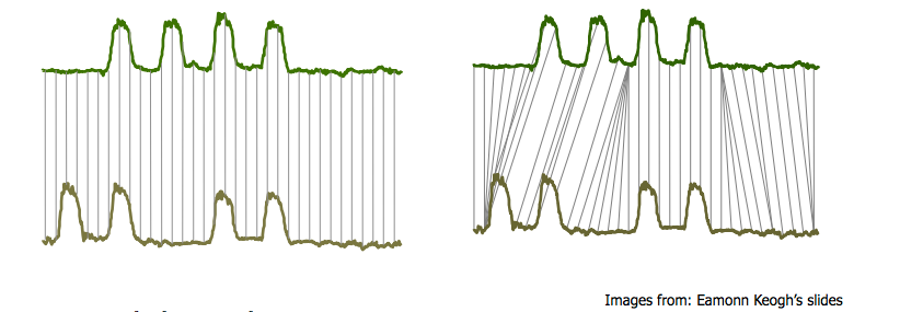
One case that arises often is something like the following: “bump hunting”

Both time series have the same key characteristics: four bumps.

But a one-to-one match (ala Euclidean distance) will not detect the similarity.

A solution to this is called dynamic time warping.

Dynamic Time Warping

The basic idea is to allow stretching or compressing of signals along the time dimension.

Classic applications

  • speech recognition
  • handwriting recognition

Specifically

  • Consider \(X = x_1, x_2, \dots, x_n\) and \(Y = y_1, y_2, \dots, y_m\).
  • We are allowed to modify each sequence by duplicating, deleting, or matching elements to form \(X'\) and \(Y'\).
  • We then search over the space of all possible alignments to find the one that minimizes the distance between \(X'\) and \(Y'\).

Visualizing DTW

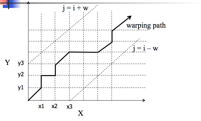
There is a simple way to visualize this algorithm.

Consider a matrix \(M\) where \(M_{ij} = |x_i - y_j|\).

\(M\) measures the amount of error we get if we match \(x_i\) with \(y_j\).

So we seek a path, starting from lower left, through \(M\) that minimizes the total error.

DTW restrictions

The basic restrictions on path are:

Monotonicity

  • The path should not go down or to the left.

Continuity

  • No elements may be skipped in a sequence.

Restrict amount of deviation from diagonal (Sakoe-Chiba constraint)

This can be solved via dynamic programming.

Dynamic Time Warping Example

Code
import numpy as np
import matplotlib.pyplot as plt

# sequences
x = [1,1,2,2,3]
y = [1,2,3,3,3]
n, m = len(x), len(y)

# build DTW table
dtw = np.full((n+1,m+1), np.inf)
dtw[0,0] = 0
for i in range(1,n+1):
    for j in range(1,m+1):
        cost = abs(x[i-1]-y[j-1])
        dtw[i,j] = cost + min(dtw[i-1,j], dtw[i,j-1], dtw[i-1,j-1])

# backtrack with tie-breaking: prefer diagonal
i,j = n,m
path = [(i-1,j-1)]
while (i>0 and j>0):
    candidates = [(i-1,j-1,"↖"), (i-1,j,"↑"), (i,j-1,"←")]
    i,j,_ = min(candidates, key=lambda s: (dtw[s[0],s[1]], ["↖","↑","←"].index(s[2])))
    if i>0 or j>0:
        path.append((i-1,j-1))
path.reverse()

# Print the fully aligned sequences
print("Original sequences:")
print(f"X = {x}")
print(f"Y = {y}")
print(f"\nDTW distance = {dtw[n,m]:.1f}")
print(f"\nOptimal alignment path (0-indexed): {path}")
print("\nFully aligned sequences:")
print("X_aligned: ", end="")
for i, j in path:
    print(f"{x[i]:2d}", end=" ")
print()
print("Y_aligned: ", end="")
for i, j in path:
    print(f"{y[j]:2d}", end=" ")
print()
print("\nAlignment mapping:")
for k, (i, j) in enumerate(path):
    print(f"Step {k}: X[{i}] = {x[i]} ↔ Y[{j}] = {y[j]}")

# plot cost matrix + path
plt.figure(figsize=(10, 4))
plt.subplot(1, 2, 1)
plt.imshow(dtw[1:,1:], origin="lower", cmap="Blues", aspect="auto")
px, py = zip(*[(pi+1,pj+1) for pi,pj in path])
plt.plot(np.array(py)-1, np.array(px)-1, 'r', linewidth=2)
plt.colorbar(label="Cumulative Cost")
plt.title("DTW Cost Matrix with Optimal Path")
plt.xlabel("Y values")
plt.ylabel("X values")

# plot aligned sequences
plt.subplot(1, 2, 2)
x_aligned = [x[i] for i, j in path]
y_aligned = [y[j] for i, j in path]
plt.plot(range(len(x_aligned)), x_aligned, 'bo-', label='X aligned', linewidth=2)
plt.plot(range(len(y_aligned)), y_aligned, 'ro-', label='Y aligned', linewidth=2)
plt.xlabel('Alignment step')
plt.ylabel('Value')
plt.title('Aligned Sequences')
plt.legend()
plt.grid(True, alpha=0.3)
plt.tight_layout()
plt.show()
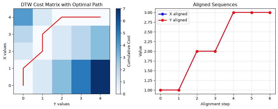
Original sequences:
X = [1, 1, 2, 2, 3]
Y = [1, 2, 3, 3, 3]

DTW distance = 0.0

Optimal alignment path (0-indexed): [(0, 0), (1, 0), (2, 1), (3, 1), (4, 2), (4, 3), (4, 4)]

Fully aligned sequences:
X_aligned:  1  1  2  2  3  3  3 
Y_aligned:  1  1  2  2  3  3  3 

Alignment mapping:
Step 0: X[0] = 1 ↔ Y[0] = 1
Step 1: X[1] = 1 ↔ Y[0] = 1
Step 2: X[2] = 2 ↔ Y[1] = 2
Step 3: X[3] = 2 ↔ Y[1] = 2
Step 4: X[4] = 3 ↔ Y[2] = 3
Step 5: X[4] = 3 ↔ Y[3] = 3
Step 6: X[4] = 3 ↔ Y[4] = 3

To explore further

See

T. Giorgino, “Computing and Visualizing Dynamic Time Warping Alignments in R: The dtw Package”, Journal of Statistical Software, 2003. link

And python packages such as:

🎯 Class Activity: DTW Concept Exploration

Task: Explore why DTW is better than Euclidean distance for time series with temporal shifts.

Given: Two simple time series:

  • Series A: [1, 2, 3, 2, 1] (peak at position 3)
  • Series B: [0, 1, 2, 3, 2, 1, 0] (peak at position 4)

Instructions:

  1. Calculate Euclidean distance between the series (pad with zeros if needed)
  2. Sketch the DTW alignment by hand:
    • Expand series A to better align with series B
  3. Calculate the Euclidean distance of the aligned series
  4. Group discussion:
    • Why does Euclidean distance of the original series fail here?
    • What real-world scenarios would benefit from DTW?

Scenarios:

  • Speech recognition (different speaking speeds)
  • Gesture recognition (different execution speeds)
  • Stock price patterns (different market timing)

From Time series to Strings

A closely related idea concerns strings.

The key point is that, like time series, strings are sequences.

Given two strings, one way to define a ‘distance’ between them is:

  • the minimum number of edit operations that are needed to transform one string into the other.

Edit operations are insertion, deletion, and substitution of single characters.

This is called edit distance or Levenshtein distance.

Example

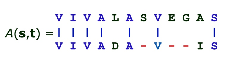
For example, given strings: s = VIVALASVEGAS and t = VIVADAVIS

we would like to

  • compute the edit distance, and
  • obtain the optimal alignment.

A dynamic programming algorithm can also be used to find this distance, and it is very similar to dynamic time-warping.

In bioinformatics this algorithm is called “Smith-Waterman” sequence alignment.

Recap

We covered the following topics

  • reviewed representations of data,
  • discussed metrics and norms,
  • discussed similarity and dissimilarity functions,
  • introduced time series,
  • feature engineering, and
  • dynamic time warping.