Recap: Hierarchical Clustering

DS701 Session 5 — Mon Sep 21, 2026

Today’s plan

• 5 min — knowledge-check review
• 20 min — highlights and Q&A (answer or pass — answering always earns credit)
• 60 min — in-class activity (small groups)
• wrap-up and cold-call check-ins

Knowledge-Check Review

KC 1: The procedure and the picture

Describe the agglomerative hierarchical clustering procedure in three steps, and say what the height at which two branches join in a dendrogram represents.

Answer.

1. Start with every point as its own cluster.
2. Merge the two closest clusters — “closest” as defined by the linkage (single, complete, average, Ward, …).
3. Repeat until one cluster remains.

The height of a join is the inter-cluster distance at the moment those two clusters were merged. Low joins are tight groups, tall joins are far-apart groups — and a horizontal cut at any height reads off one flat clustering.

KC 2: min versus max

Single linkage defines the distance between two clusters as the distance between their closest pair of points; complete linkage uses their farthest pair. Explain, from these definitions alone, why single linkage tends to produce long chains that can connect two well-separated groups through a few noise points, and why complete linkage tends toward compact clusters of similar diameter.

Single — one close cross pair is enough to merge, so a cluster grows by absorbing whatever is nearest to any member. A string of noise points, each close to the next, stitches two distant groups together: chaining. (Same property lets it follow a crescent.)

Complete — a merge is charged the farthest cross pair, i.e. the diameter of the merged cluster. Merging anything elongated or already large is expensive, so clusters stay compact and similar in size; a thin bridge of points does not shrink the max — but one far outlier inflates it.

KC 3: When the client will not tell you \(k\)

A client asks you to segment their customers but cannot tell you how many segments they want. Explain why hierarchical clustering is a natural fit here compared to \(k\)-means, and how you would still get a concrete number of segments out of it.

Why hierarchical: \(k\)-means needs \(k\) before it runs and returns one partition. Hierarchical clustering does not decide \(k\) — the dendrogram holds a nested clustering at every scale, so all candidate segmentations are visible at once (and the tree may itself be meaningful, like a taxonomy).

Getting a number anyway: cut the tree —

• at a height where there is a large gap between successive merges,
• or flatten to \(k = 2, 3, \dots\) with fcluster and score each cut (silhouette — first peak, as on the newsgroups),
• or at the granularity the business can act on.

KC 4: Manually Build H-Cluster

On the figures in the exercise of the lecture draw out the clusters formed via an agglomerative (bottoms-up) hierarchical clustering process. Draw out the corresponding dendrogram as well. You can just visually assess the distances to pick the clusters and approximate the heights on the dendrogram.

Highlights

Not one partition — a whole tree

Last session: a strict partition — every point in exactly one of \(k\) clusters, \(k\) chosen in advance.

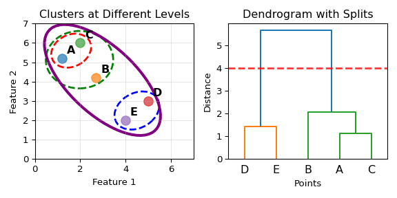
• But “how many clusters?” often has several honest answers, depending on scale.
• A hierarchical clustering returns nested clusters organised as a tree.
• The dendrogram records the containment relations: leaves are points, each join is a merge, height is the distance at which it happened.
• It does not decide the number of clusters — you cut it, at any level, afterwards.

The agglomerative procedure

1. Initialise: each point is its own cluster; compute the pairwise distance matrix if not given.
2. Merge the two closest clusters (per the linkage and the metric).
3. Update the distances from the new cluster to all remaining clusters.
4. Repeat 2–3 until one cluster remains.

The output is a linkage matrix of shape \((n-1, 4)\) — one row per merge:

\[ [\ \text{idx}_1,\ \text{idx}_2,\ \text{distance},\ \text{count}\ ] \]

Indices \(0 \dots n-1\) are original points; indices \(n, n+1, \dots\) are the clusters created by earlier rows. scipy.cluster.hierarchy.linkage produces it; dendrogram draws it; fcluster cuts it.

Everything hinges on the linkage

Distance between two clusters \(C_i, C_j\) — three natural choices, plus one borrowed from \(k\)-means:

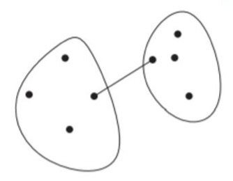
Single \[\min_{x\in C_i,\,y\in C_j} d(x,y)\]

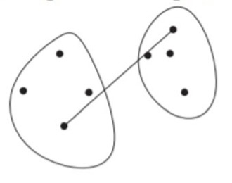
Complete \[\max_{x\in C_i,\,y\in C_j} d(x,y)\]

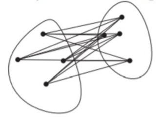
Average \[\frac{1}{|C_i||C_j|}\sum_{x\in C_i,\,y\in C_j} d(x,y)\]

Ward: the increase in within-cluster sum of squares if \(C_i\) and \(C_j\) were merged — merge the pair that hurts the \(k\)-means objective least. A hierarchical, greedy \(k\)-means.

Same data, four personalities

linkage	good at	fails when	shape bias
single	connected, odd shapes (moons, rings); unequal sizes	a few noise points bridge two groups → chaining	none
complete	balanced, similar-diameter clusters; ignores bridges	one far outlier dominates the max	compact / spherical
average	a compromise; less noise- and outlier-sensitive	—	elliptical
ward	like \(k\)-means: robust, tidy blobs	non-convex shapes; needs Euclidean features	elliptical

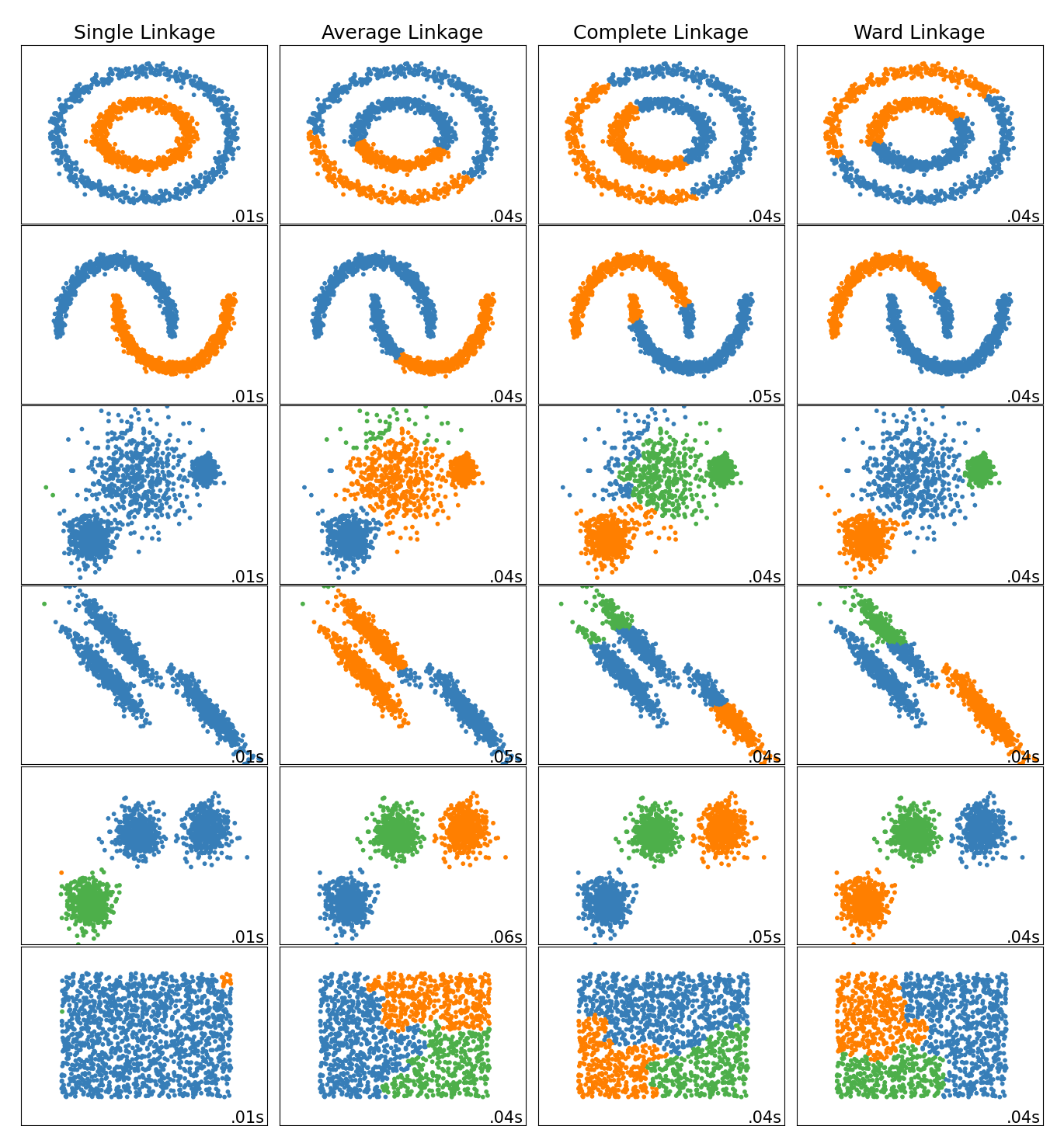
Comparison of linkages

No linkage wins every row — the linkage is a modelling choice about what a cluster should look like.

Scikit-Learn Comparison

Cutting the tree

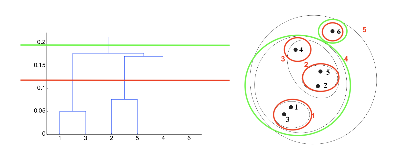
Two ways to flatten a hierarchy:

• by height — fcluster(Z, h, criterion="distance"): every merge below \(h\) is done. The red and green lines are two such cuts.
• by count — fcluster(Z, k, criterion="maxclust"): at most \(k\) clusters.
• Where to cut? Look for a large gap between successive merge heights, or sweep \(k\) and score each cut (silhouette), or ask what the clusters are for.

Heights are only comparable within one dendrogram — single-linkage heights are nearest-neighbour distances, Ward’s accumulate squared error.

Hierarchical vs. partitional

	\(k\)-means (partitional)	agglomerative (hierarchical)
needs \(k\) up front	yes	no — cut afterwards
output	one partition	a tree of nested partitions
input	points in \(\mathbb{R}^d\) (needs means)	feature matrix or any distance / similarity matrix
cluster shape	spherical Voronoi cells	depends on linkage
cost	cheap, iterative	\(O(n^2)\) memory, \(O(n^2 \log n)\) time — fine for thousands, not millions
repeatability	random init	deterministic

Reach for a dendrogram when you do not know \(k\), when the nesting itself is the answer (taxonomies), or when all you have is a distance matrix.

Today’s activity: the same data, both tools, and three kinds of mess — find out for yourself which survives what.

Going deeper

Full lecture notes: Hierarchical Clustering

• How Many Clusters? — the same data at 3, 4, 5 and 6 clusters
• Example: Dendrogram — five points, built up merge by merge
• Hierarchical Clustering Algorithms — agglomerative vs divisive; the linkage matrix
• Defining Cluster Proximity — single, complete, average, and their strengths and failures on moons and blobs
• Ward’s Distance
• Selecting the Number of Clusters — silhouette on the newsgroups tree
• Comparison of Linkages — scikit-learn’s side-by-side figure
• Cluster evaluation (ARI, silhouette) and real-data practice: Clustering in Practice

In-Class Activity

Activity: dendrograms on real data, then make it messy

Goal: build and read dendrograms for four linkages on a real dataset, cut them into flat clusters, then inject a unit change, two outliers and a chaining bridge and watch which linkages survive — and whether \(k\)-means would have been fine all along.

• Work in groups of 2–3. Open your section’s notebook.
• Parts marked (autograded) are submitted to Gradescope; the rest is participation.
• Staff will circulate — be ready to explain any part of your work.
• Dependencies: numpy, pandas, matplotlib, scipy, scikit-learn.

The activity notebook goes live on the day of the lecture. Colab is optional — you can also open it on GitHub and run it locally.