Recap: Probabilistic Modeling
DS701 Session 6 — Wed Sep 23, 2026
Idea 1 — fit, then check
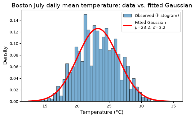
Fitting is cheap. Checking is what makes it a model rather than an assumption.
- Overlay the fitted density on the histogram.
- Compare what the model predicts with what you count: within \(1\sigma\): model \(0.683\), data \(0.664\); within \(2\sigma\): \(0.954\) vs \(0.966\).
- Test an implied property: for a Poisson, mean \(=\) variance (\(0.610\) vs \(0.608\)).
- Then use it: \(P(T > 30\,°\text{C})\) — model \(0.0165\), data \(0.0117\). Least trustworthy in the tails.
Idea 1, continued — when the check fails, believe the check
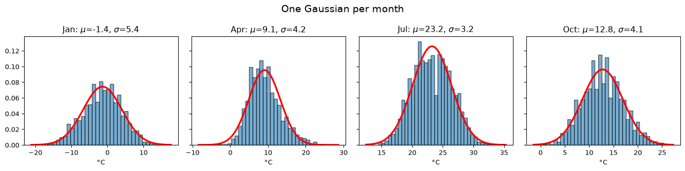
- One Gaussian per month: parameters differ a lot, and April shows a warm tail the bell cannot follow. The check tells you where the model is trustworthy.
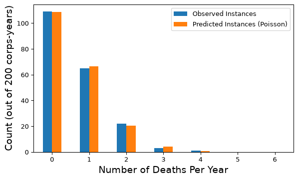
- Horse kicks: \(\hat\lambda = 0.61\) deaths per corps-year predicts \(108.7 / 66.3 / 20.2 / 4.1 / 0.6\) corps-years with \(0/1/2/3/4\) deaths; observed \(109 / 65 / 22 / 3 / 1\).
- So the years with 3 or 4 deaths are exactly what randomness looks like at a constant rate — no story needed.
Idea 2 — MLE: maximize the likelihood of what you saw
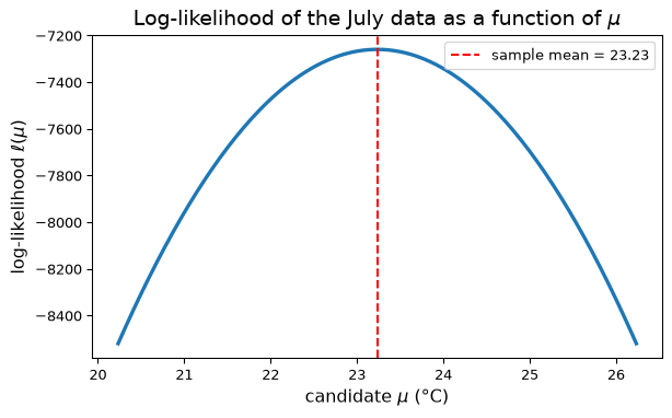
The Gaussian log-likelihood of the July data as \(\mu\) varies (\(\sigma\) fixed) — it peaks exactly at the sample mean.
The recipe, for any model:
- Write the probability of the observed data as a function of the parameters (independence \(\Rightarrow\) a product).
- Take the log (product \(\to\) sum; same argmax).
- Maximize: set derivatives to zero.
\[ \ell(\mu,\sigma^2) = -\tfrac{N}{2}\log(2\pi\sigma^2) - \tfrac{1}{2\sigma^2}\textstyle\sum_n (x_n-\mu)^2 \] \[ \frac{\partial \ell}{\partial \mu} = \frac{1}{\sigma^2}\sum_n (x_n-\mu) = 0 \;\Rightarrow\; \hat\mu = \frac{1}{N}\sum_n x_n \]
Idea 3 — covariance shapes the multivariate Gaussian
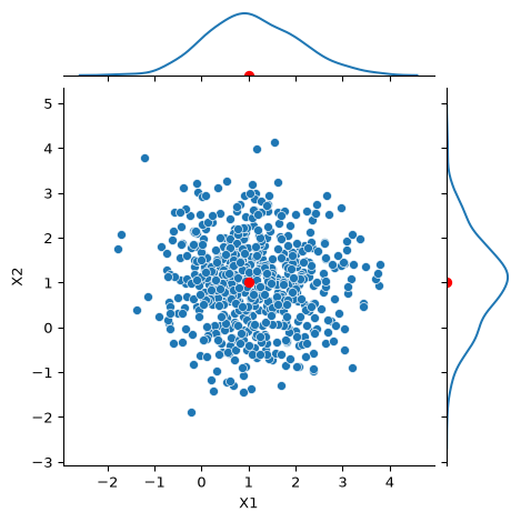
\(\Sigma = \begin{bmatrix}1&0\\0&1\end{bmatrix}\)
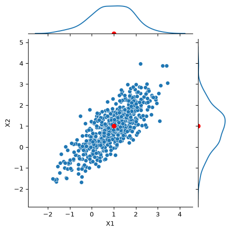
\(\Sigma = \begin{bmatrix}1&0.8\\0.8&1\end{bmatrix}\)
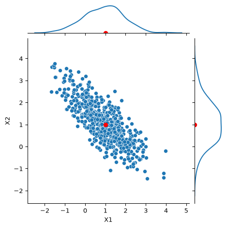
\(\Sigma = \begin{bmatrix}1&-0.8\\-0.8&1\end{bmatrix}\)
- \(\mathbf{X} \sim \mathcal{N}(\mathbf{\mu}, \Sigma)\): same two parameters as before, except the mean is a vector and the variance is a matrix, \(\Sigma_{ij} = \text{Cov}(X_i, X_j)\).
- \(\text{Cov}(X,Y) = E[(X-\mu_X)(Y-\mu_Y)]\); correlation \(\rho = \text{Cov}/(\sigma_X\sigma_Y) \in [-1,1]\). \(\rho = 0\) means no linear relationship — not independence.
- The off-diagonal stretches circles into tilted ellipses; the marginals stay Gaussian. (TSLA/NVDA: \(\rho \approx 0.86\) — a cloud along the diagonal, and arguably not one Gaussian. Hold that thought for GMMs.)
Idea 4 — the CLT: sample means become Gaussian, and narrow
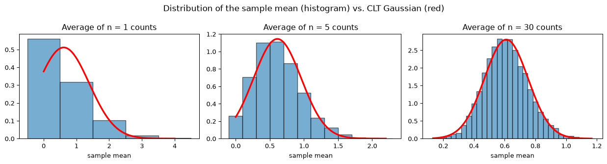
- Average \(n\) horse-kick counts (definitely not Gaussian), repeat 5000 times, histogram the averages.
- Any distribution with finite variance: as \(n\) grows the sample mean is \(\approx \mathcal{N}(\mu, \sigma^2/n)\).
- Two things happen at once: the shape becomes a bell, and the spread shrinks — the standard error is \(\sigma/\sqrt{n}\).
Idea 4, continued — a confidence interval, and how to read it
\[ \bar{x} \;\pm\; z_{1-\alpha/2}\,\frac{s}{\sqrt{n}}, \qquad z_{0.975} \approx 1.96 \]
- All July days (\(n = 2821\)): \([23.12,\ 23.35]\) °C. July 2020 alone (\(n = 31\)): \([22.83,\ 25.28]\) °C.
- The 95% is about the procedure: repeat the experiment many times and about 95% of the intervals cover the true mean. Any particular interval either does or does not.
- Width \(\propto 1/\sqrt{n}\): to halve it you need four times the data.
- It quantifies uncertainty in the mean only — individual days still range over \(\mu \pm 2\sigma\).
- Assumes independent samples; hot days cluster, so the honest interval is a bit wider.
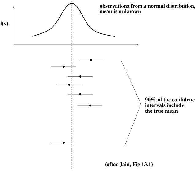
Each bar is the interval from one dataset; most cover the true mean, a few miss.
Activity: fit, check — then simulate what the theorems promise
Goal: run the recipe yourself on a month of Boston temperatures (Gaussian, MLE by hand and with scipy) and on the horse-kick counts (Poisson), check each fit and use it — then, as the stretch, treat your fitted Poisson as a known population and watch the Law of Large Numbers, the Central Limit Theorem, and the coverage of your own 95% confidence intervals.
- Work in groups of 2–3. Sections A1 and B1 get different months, corps, and seeds — open your section’s notebook.
- Parts marked (autograded) are submitted to Gradescope; the rest is participation.
- Staff will circulate — be ready to explain any part of your work.
- Dependencies:
numpy,pandas,matplotlib,scipyonly.


The activity notebook goes live on the day of the lecture. Colab is optional — you can also open it on GitHub and run it locally.