Recap: Soft Clustering with Gaussian Mixture Models
DS701 Session 7 — Mon Sep 28, 2026
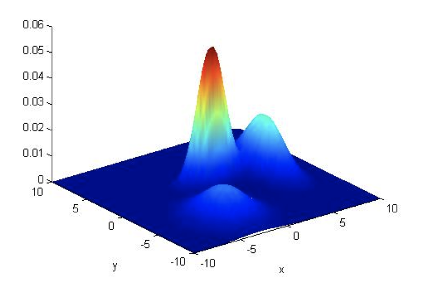
The model is a recipe for making data
For each of the \(n\) points, independently:
- roll a \(K\)-sided die with face probabilities \(\pi_1, \dots, \pi_K\) — that is the latent label \(z_i\);
- draw \(x_i\) from the Gaussian for that face, \(\mathcal{N}(\mu_{z_i}, \Sigma_{z_i})\).
Forget the die roll and you get the mixture density \[ p(x \mid \theta) = \sum_{k=1}^{K} \pi_k\, \mathcal{N}(x \mid \mu_k, \Sigma_k). \]
Clustering = running the recipe backwards: given only the \(x_i\), recover \(\theta\) and say how each point was probably rolled.
E-step: Bayes’ rule, one point at a time
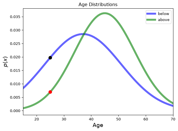
Age 25 in the income example. Black dot: density under below; red dot: density under above.
\[ P(\text{above} \mid 25) = \frac{\text{red}\cdot P(\text{above})}{\text{red}\cdot P(\text{above}) + \text{black}\cdot P(\text{below})} \]
Same thing for every point \(i\) and component \(k\): \[ \gamma_{ik} = \frac{\pi_k\, \mathcal{N}(x_i \mid \mu_k, \Sigma_k)}{\sum_{j} \pi_j\, \mathcal{N}(x_i \mid \mu_j, \Sigma_j)} \]
prior \(\pi_k\), likelihood \(\mathcal{N}(\cdot)\), evidence = the mixture density. Rows sum to 1.
GMM vs. \(k\)-means, side by side
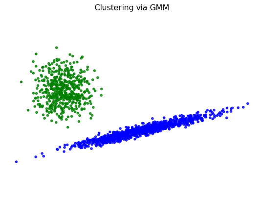
covariance_type="full"
- Same two-phase loop; soft vs. hard assignment is the practical difference (“soft \(k\)-means”).
- The GMM’s assumption is explicit — a mixture of Gaussians — so it can be inspected, tightened, or swapped. \(k\)-means only declared an objective.
- Here the explicit covariance is what saves the thin cluster’s tip: nearest-center distance hands it to the blob.
Activity: EM by hand, then soft vs. hard — visualized
Goal: implement the E-step and M-step yourself on a 1-D two-component mixture, iterate while watching the log-likelihood climb, check against sklearn.mixture.GaussianMixture — then go to 2-D: responsibilities as color intensity next to \(k\)-means’ straight boundaries, the four covariance types as fitted ellipses, and one point the GMM calls 50/50.
- Work in groups of 2–3.
- Parts marked (autograded) are submitted to Gradescope; the rest is participation.
- Staff will circulate — be ready to explain any part of your work.
- Dependencies:
numpy,scipy,matplotlib,scikit-learnonly.
Section A1: 

Section B1:
The activity notebook goes live on the day of the lecture. Colab is optional — you can also open it on GitHub and run it locally.