GMM Appendix C: Deriving the E-Step: From Indicators to Responsibilities
Starting Point: The Complete Data Log-Likelihood1
Appendix B showed that if the cluster assignments \(z_1, \ldots, z_n\) were known, the log-likelihood of the data and the assignments together would be
where the indicator \(\mathbb{1}(z_i = k)\) is \(1\) if \(z_i = k\) and \(0\) otherwise, so for each point exactly one term of the inner sum survives. No sum sits inside a log, which is what makes this form easy to maximize.
The E-Step: Taking Expectations
The problem is that we don’t observe \(Z\), so we can’t compute the complete data log-likelihood directly. The EM algorithm solves this by taking the expected value of the complete data log-likelihood with respect to the distribution of \(Z\) given \(X\) and the current parameters \(\theta^{(t)}\).
The Q-Function
The lecture calls the result the expected complete-data log-likelihood; its standard name is the \(Q\)-function:
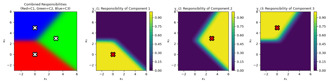
import matplotlib.pyplot as plt# Generate a grid of pointsx_range = np.linspace(-3, 6, 100)y_range = np.linspace(-3, 8, 100)X_grid, Y_grid = np.meshgrid(x_range, y_range)grid_points = np.column_stack([X_grid.ravel(), Y_grid.ravel()])# Compute responsibilities for every grid point at once: one pdf call per componentnumerators = np.column_stack([ pi[k] * multivariate_normal.pdf(grid_points, mean=mu[k], cov=Sigma[k])for k inrange(3)])responsibilities = numerators / numerators.sum(axis=1, keepdims=True)# Reshape for plottinggamma_1 = responsibilities[:, 0].reshape(X_grid.shape)gamma_2 = responsibilities[:, 1].reshape(X_grid.shape)gamma_3 = responsibilities[:, 2].reshape(X_grid.shape)# Create RGB image where each color represents a clusterrgb_image = np.zeros((X_grid.shape[0], X_grid.shape[1], 3))rgb_image[:, :, 0] = gamma_1 # Red for cluster 1rgb_image[:, :, 1] = gamma_2 # Green for cluster 2rgb_image[:, :, 2] = gamma_3 # Blue for cluster 3# Plotfig, axes = plt.subplots(1, 4, figsize=(14, 3.6))# RGB combined viewaxes[0].imshow(rgb_image, extent=[x_range[0], x_range[-1], y_range[0], y_range[-1]], origin='lower', aspect='auto')axes[0].scatter(mu[:, 0], mu[:, 1], c='white', s=200, marker='X', edgecolors='black', linewidths=2)axes[0].set_title('Combined Responsibilities\n(Red=C1, Green=C2, Blue=C3)', fontsize=10)axes[0].set_xlabel('x₁')axes[0].set_ylabel('x₂')# Individual responsibility mapsfor k inrange(3): gamma_k = responsibilities[:, k].reshape(X_grid.shape) im = axes[k+1].contourf(X_grid, Y_grid, gamma_k, levels=20, cmap='viridis') axes[k+1].scatter(mu[k, 0], mu[k, 1], c='red', s=200, marker='X', edgecolors='black', linewidths=2) axes[k+1].set_title(f'γ_i{k+1}: Responsibility of Component {k+1}', fontsize=10) axes[k+1].set_xlabel('x₁') axes[k+1].set_ylabel('x₂') plt.colorbar(im, ax=axes[k+1])plt.tight_layout()plt.show()
Key Properties of Responsibilities
1. Normalization
For each point \(i\): \[
\sum_{k=1}^{K} \gamma_{ik} = 1
\]
This follows from the law of total probability.
Code
# Verify normalizationprint("Verification that responsibilities sum to 1:")for i inrange(5): point = grid_points[i] likelihoods = np.array([ multivariate_normal.pdf(point, mean=mu[k], cov=Sigma[k])for k inrange(3) ]) numerators = pi * likelihoods gamma = numerators / np.sum(numerators)print(f"Point {i}: sum of γ = {np.sum(gamma):.10f}")
Verification that responsibilities sum to 1:
Point 0: sum of γ = 1.0000000000
Point 1: sum of γ = 1.0000000000
Point 2: sum of γ = 1.0000000000
Point 3: sum of γ = 1.0000000000
Point 4: sum of γ = 1.0000000000
2. Soft Assignment
\(\gamma_{ik} = 1\): point \(i\) definitely belongs to cluster \(k\)
\(\gamma_{ik} = 0\): point \(i\) definitely does not belong to cluster \(k\)
3. Relationship to Hard Assignment and \(k\)-Means
A hard assignment keeps only the winner, \(z_i = \arg\max_k \gamma_{ik}\), and throws the rest of the row away; EM keeps the whole row. Replacing the E-step by this argmax gives “hard EM” (also called classification EM). It becomes \(k\)-means exactly when every component has the same weight and the same spherical covariance \(\sigma^2 I\): then \(\arg\max_k \gamma_{ik}\) is the nearest centre, and the M-step means are plain per-cluster averages. That is the lecture’s remark that \(k\)-means is EM with every \(\gamma_{ik} \in \{0, 1\}\).
Code
# Compare soft vs hard assignmentstest_point = np.array([1.5, 1.5])likelihoods = np.array([ multivariate_normal.pdf(test_point, mean=mu[k], cov=Sigma[k])for k inrange(3)])numerators = pi * likelihoodsgamma = numerators / np.sum(numerators)print(f"Test point: {test_point}")print(f"\nSoft assignment (EM):")for k inrange(3):print(f" Cluster {k+1}: {gamma[k]:.4f}")print(f"\nHard assignment (argmax):")hard_assignment = np.argmax(gamma) +1print(f" Cluster {hard_assignment}")
Key insight: Since we don’t know which cluster generated each point, we replace the binary indicator \(\mathbb{1}(z_i = k)\) with its expected value under the posterior distribution, which is the probability (responsibility) \(\gamma_{ik}\).