We now consider applications of the Singular Value Decomposition (SVD).
SVD is “the Swiss Army Knife of Numerical Linear Algebra.”
Dianne O’Leary, MMDS ’06 (Workshop on Algorithms for Modern Massive Data Sets)
Lecture Organization
In this lecture we:
review the linear algebra the SVD is built on: orthonormal vectors, eigenvalues of symmetric matrices, and matrix rank;
define the SVD, see where its three factors come from, and work one out by hand;
prove what it is good for: the SVD gives the best low rank approximation to any matrix (the Eckart–Young theorem);
apply it to data matrices from four applications
internet traffic data
social media data
image data
movie data
The other big use of the SVD, dimensionality reduction (PCA), is the subject of the next lecture.
Linear Algebra Prerequisites
Notation
Throughout this lecture a matrix \(A \in \mathbb{R}^{m\times n}\) has \(m\) rows and \(n\) columns, and we assume \(m > n\): more rows than columns.
For a data matrix this means rows are observations and columns are features, with more observations than features — the common case.
Note that this is the matrix-theory convention. In the regression lectures we wrote the data matrix as \(n \times p\) with \(n\) observations; here \(m\) plays the role of \(n\) and \(n\) the role of \(p\).
Orthonormal Vectors and Orthogonal Matrices
A set of vectors \(\{\mathbf{q}_1, \dots, \mathbf{q}_n\}\) is orthonormal if the vectors are mutually perpendicular and each has unit length:
\[
\mathbf{q}_i^T \mathbf{q}_j = \begin{cases} 1 & i = j \\ 0 & i \neq j. \end{cases}
\]
Collect them as the columns of a matrix \(Q\). Then the entries of \(Q^TQ\) are exactly these dot products, so
\[
Q^T Q = I.
\]
If \(Q\) is also square, then \(Q Q^T = I\) as well: \(Q\) is an orthogonal matrix and its inverse is simply its transpose, \(Q^{-1} = Q^T\).
Orthogonal matrices preserve lengths and angles: \(\Vert Q\mathbf{x}\Vert = \Vert\mathbf{x}\Vert\). Geometrically they are rotations and reflections. A familiar example is the \(2\times 2\) rotation matrix
For a square matrix \(S \in \mathbb{R}^{n\times n}\), a nonzero vector \(\mathbf{x}\) is an eigenvector with eigenvalue\(\lambda\) if
\[
S\mathbf{x} = \lambda \mathbf{x}.
\]
\(S\) does not change the direction of \(\mathbf{x}\); it only stretches it by the factor \(\lambda\).
For example,
\[
S = \begin{bmatrix}2 & 1\\1 & 2\end{bmatrix}
\]
has eigenvalues \(\lambda_1 = 3\) and \(\lambda_2 = 1\), with eigenvectors \(\mathbf{x}_1 = \frac{1}{\sqrt{2}}\begin{bmatrix}1\\1\end{bmatrix}\) and \(\mathbf{x}_2 = \frac{1}{\sqrt{2}}\begin{bmatrix}1\\-1\end{bmatrix}\).
The matrix \(S\) above is symmetric: \(S = S^T\). Symmetric matrices have two properties we will rely on (this is the spectral theorem):
all \(n\) eigenvalues are real, and
the eigenvectors can be chosen to be orthonormal.
Collecting the eigenvectors into an orthogonal matrix \(Q\) and the eigenvalues into a diagonal matrix \(\Lambda\) gives the eigendecomposition
\[
S = Q \Lambda Q^T.
\]
For the example above, \(Q = \frac{1}{\sqrt{2}}\begin{bmatrix}1 & 1\\ 1 & -1\end{bmatrix}\) and \(\Lambda = \begin{bmatrix}3 & 0\\ 0 & 1\end{bmatrix}\). Notice that the two eigenvectors are indeed perpendicular.
One more fact. If \(S = B^TB\) for some matrix \(B\), then every eigenvalue is nonnegative, because for a unit eigenvector \(\mathbf{x}\)
\[
\lambda = \mathbf{x}^T S \mathbf{x} = \mathbf{x}^T B^T B \mathbf{x} = \Vert B\mathbf{x}\Vert^2 \geq 0.
\]
Keep \(B^TB\) in mind — it is about to reappear as \(A^TA\).
Matrix Rank
Let \(A\in\mathbb{R}^{m\times n}\) be a real matrix with \(m>n\).
The rank of \(A\) is the number of linearly independent rows or columns of the matrix.
The largest value that a matrix rank can take is \(\min(m,n)\). Since we assumed \(m>n\), the largest value of the rank is \(n\).
If the matrix \(A\) has rank equal to \(n\), then we say it is full rank.
However, it can happen that the rank of a matrix is less than \(\min(m,n)\). In this case we say that \(A\) is rank-deficient.
Matrix Rank and Column Space
The dimension of the column space of \(A\) is the smallest number of vectors that suffice to construct the columns of \(A\).
And it is equal to the rank of the matrix.
If the dimension of the column space is \(k\), then there exists a set of vectors \(\{\mathbf{c}_1, \mathbf{c}_2, \dots, \mathbf{c}_k\}\) such that every column \(\mathbf{a}_i\) of \(A\) can be expressed as:
The vectors \(\mathbf{x}\) with \(A\mathbf{x} = \mathbf{0}\) form the null space of \(A\). When \(A\) has rank \(k\), the null space has dimension \(n - k\).
To store a matrix \(A \in \mathbb{R}^{m\times n}\) we need to store \(mn\) values.
However, if \(A\) has rank \(k\), it can be factored as \(A = CR\), \[
A =
\begin{bmatrix}
\bigg| & \bigg| & & \bigg| \\
\mathbf{c}_1 & \mathbf{c}_2 & \dots & \mathbf{c}_k \\
\bigg| & \bigg| & & \bigg|
\end{bmatrix}
\begin{bmatrix}
\vert & \vert & & \vert \\
\mathbf{r}_1 & \mathbf{r}_2 & \dots & \mathbf{r}_n \\
\vert & \vert & & \vert
\end{bmatrix}
\]
where \(C \in \mathbb{R}^{m\times k}\) and \(R \in \mathbb{R}^{k \times n}\).
This requires \(k(m+n)\) values, which could be much smaller than \(mn\) when \(k\) is small, e.g. \(k < \frac{mn}{m+n}\).
The Singular Value Decomposition
Singular Vectors and Values
For
\[
A\in\mathbb{R}^{m\times n} \text{ with } m>n \text{ and rank } k,
\]
there exists an orthonormal set of vectors \(\{\mathbf{v}_1, \mathbf{v}_2, \dots, \mathbf{v}_n\}\) with \(\mathbf{v}_i \in \mathbb{R}^n\)
and an orthonormal set of vectors \(\{\mathbf{u}_1, \mathbf{u}_2, \dots, \mathbf{u}_n\}\) with \(\mathbf{u}_i \in \mathbb{R}^m\)
where \(\sigma_1 \geq \sigma_2 \geq \dots \geq \sigma_k > 0\) are the singular values of \(A\).
\(\mathbf{v}_{k+1}, \ldots, \mathbf{v}_n\) are an orthonormal basis for the null space of \(A\), and
\(\mathbf{u}_{k+1}, \ldots, \mathbf{u}_n\) are any unit vectors orthogonal to \(\mathbf{u}_1, \ldots, \mathbf{u}_k\) (and to each other). They are multiplied by zero, so their choice does not matter.
Compare with an eigenvector: \(A\) maps \(\mathbf{v}_i\) to a different vector \(\mathbf{u}_i\), living in a different space (\(\mathbb{R}^m\) rather than \(\mathbb{R}^n\)), scaled by \(\sigma_i\). That is why this works for rectangular matrices, where eigenvectors are not even defined.
Singular Value Decomposition
We can collect the vectors \(\mathbf{v}_i\) into a matrix \(V\) and the vectors \(\mathbf{u}_i\) into a matrix \(U\). \[
A
\begin{bmatrix}
\vert & \vert & & \vert \\
\mathbf{v}_1 & \mathbf{v}_2 & \dots & \mathbf{v}_n \\
\vert & \vert & & \vert
\end{bmatrix} =
\begin{bmatrix}
\vert & \vert & & \vert \\
\mathbf{u}_1 & \mathbf{u}_2 & \dots & \mathbf{u}_n \\
\vert & \vert & & \vert
\end{bmatrix}
\left[
\begin{array}{c|c}
\begin{matrix}
\sigma_1 & \cdots & 0 \\
\vdots & \ddots & \vdots \\
0 & \cdots & \sigma_k
\end{matrix}
&
\mathbf{0}
\\
\hline
\mathbf{0} & \mathbf{0}
\end{array}
\right]
.
\]
We call the \(\mathbf{v}_i\) the right singular vectors and the \(\mathbf{u}_i\) the left singular vectors.
Singular Value Decomposition
And because \(V\) is an orthogonal matrix, we have \(V V^T = I\), so we can right multiply both sides by \(V^T\) to get
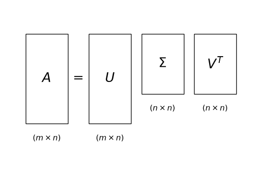
The SVD of a matrix \(A\in\mathbb{R}^{m\times n}\) (where \(m>n\)) is
\[
A = U\Sigma V^{T},
\]
where
\(U\) has dimension \(m\times n\). The columns of \(U\) are orthonormal, so \(U^TU = I_n\). The columns of \(U\) are the left singular vectors.
\(\Sigma\) has dimension \(n\times n\). The only non-zero values are on the main diagonal and they are nonnegative real numbers \(\sigma_1\geq \sigma_2 \geq \ldots \geq \sigma_k > 0\) and \(\sigma_{k+1} = \ldots = \sigma_n = 0\). These are called the singular values of \(A\).
\(V\) has dimension \(n \times n\). The columns of \(V\) are orthonormal, so \(V\) is an orthogonal matrix. The columns of \(V\) are the right singular vectors.
Thin versus full SVD
This is the thin (or economy) SVD, and it is the one we use throughout. The full SVD pads \(U\) with \(m-n\) more orthonormal columns to make it a square \(m\times m\) orthogonal matrix, and pads \(\Sigma\) with \(m-n\) rows of zeros to make it \(m\times n\). The extra columns of \(U\) multiply only zeros, so the two versions give the same \(A\). np.linalg.svd returns the full version by default; pass full_matrices=False to get the thin one, which is what you want for data matrices (\(1008\times 1008\) versus \(1008\times 121\) for the traffic matrix below).
The SVD of a matrix always exists. The next slide shows why.
The SVD itself dates to Beltrami and Jordan in the 1870s. That its truncation gives the best low-rank approximation was proven in 1936 by Carl Eckart and Gale Young.
The singular values are uniquely determined.
When the singular values are distinct, the left and right singular vectors are uniquely determined up to sign: replacing \(\mathbf{u}_i, \mathbf{v}_i\) by \(-\mathbf{u}_i, -\mathbf{v}_i\) leaves \(\sigma_i\mathbf{u}_i\mathbf{v}_i^T\) unchanged. (Repeated singular values allow more freedom, as the \(\mathbf{u}_i\) beyond the rank already showed.)
Where do \(U\), \(\Sigma\), \(V\) come from?
Suppose \(A = U\Sigma V^T\). Then, using \(U^TU = I\),
\[
A^TA = (U\Sigma V^T)^T (U\Sigma V^T) = V \Sigma U^T U \Sigma V^T = V \Sigma^2 V^T.
\]
Look at what this says. \(A^TA\) is a square (\(n\times n\)) symmetric matrix, and \(V\Sigma^2V^T\) is exactly the eigendecomposition \(Q\Lambda Q^T\) of the previous section:
the right singular vectors \(\mathbf{v}_i\) are the eigenvectors of \(A^TA\), and
the squared singular values \(\sigma_i^2\) are its eigenvalues: \(\sigma_i = \sqrt{\lambda_i(A^TA)}\).
Once we have \(\mathbf{v}_i\) and \(\sigma_i\), the defining relation \(A\mathbf{v}_i = \sigma_i\mathbf{u}_i\) hands us the left singular vectors:
In practice np.linalg.svd does not form \(A^TA\) (squaring the matrix squares its condition number); it works on \(A\) directly. But the recipe above is how you compute a small SVD by hand, and it is the identity that connects the SVD to PCA next lecture.
the matrix from the eigenvalue example: \(\lambda_1 = 3\), \(\lambda_2 = 1\), with eigenvectors \(\mathbf{v}_1 = \frac{1}{\sqrt{2}}\begin{bmatrix}1\\1\end{bmatrix}\), \(\mathbf{v}_2 = \frac{1}{\sqrt{2}}\begin{bmatrix}1\\-1\end{bmatrix}\).
Step 2: singular values.\(\sigma_1 = \sqrt{3}\), \(\sigma_2 = \sqrt{1} = 1\). Both are non-zero, so \(A\) has rank 2 (full rank).
Step 3: left singular vectors, \(\mathbf{u}_i = A\mathbf{v}_i/\sigma_i\).
Two sanity checks we will justify shortly: \(\Vert A\Vert_F^2 = 1+1+0+1+1+0 = 4 = 3 + 1 = \sigma_1^2 + \sigma_2^2\), and the number of non-zero singular values (2) equals the rank.
# The same vectors from the eigendecomposition of A^T Alam, V = np.linalg.eigh(A.T @ A) # eigh: eigenvalues in ascending orderprint("eigenvalues of A^T A:", lam[::-1], " -> sqrt:", np.sqrt(lam[::-1]))print("eigenvectors (columns):\n", V[:, ::-1])
Note that numpy returned \(\mathbf{u}_1\) and \(\mathbf{v}_1\) with the opposite sign from our hand computation. Both are correct: the singular vectors are only determined up to sign, and flipping \(\mathbf{u}_1\) and \(\mathbf{v}_1\) together leaves \(\sigma_1 \mathbf{u}_1\mathbf{v}_1^T\) unchanged.
The SVD as a Geometric Picture
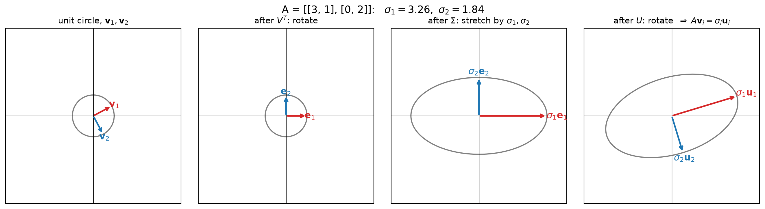
\(A = U\Sigma V^T\) says that multiplying by \(A\) is three simple steps: rotate (by \(V^T\)), stretch along the axes (by \(\Sigma\)), rotate again (by \(U\)).
Multiplying the unit circle by \(A\), one factor at a time. \(V^T\) rotates \(\mathbf{v}_1, \mathbf{v}_2\) onto the coordinate axes, \(\Sigma\) stretches the axes by \(\sigma_1, \sigma_2\), and \(U\) rotates the result so the axes land on \(\mathbf{u}_1, \mathbf{u}_2\). Unlike an eigenvector, \(\mathbf{v}_i\)changes direction: it ends up along \(\mathbf{u}_i\).
Outer Products
The SVD can also be represented as a sum of outer products
\[
A = \sum_{i=1}^{n} \sigma_{i}\mathbf{u}_i\mathbf{v}_{i}^{T},
\]
where \(\mathbf{u}_i, \mathbf{v}_{i}\) are the \(i\)-th columns of \(U\) and \(V\), respectively.
Only the first \(k\) terms are non-zero, since \(\sigma_{k+1} = \dots = \sigma_n = 0\). In other words, the rank of \(A\) is the number of non-zero singular values.
Outer Products, continued
An outer product of a \(m\times 1\) vector and a \(1\times n\) vector is a \(m\times n\) matrix.
Here \(u_{ij}\) denotes the \(j\)-th entry of \(\mathbf{u}_i\), and likewise \(v_{ij}\) is the \(j\)-th entry of \(\mathbf{v}_i\).
It is a rank-1 matrix. How can you tell?
Alternate Interpretation:
The SVD decomposes \(A\) into a linear combination of rank-1 matrices.
The singular value tells us the weight (contribution) of each rank-1 matrix to the matrix \(A\).
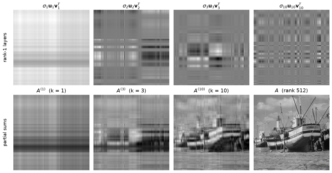
Here is what that looks like for a photograph (a \(512\times 512\) matrix of gray levels that we will come back to later in the lecture).
Top row: individual rank-1 layers \(\sigma_i\mathbf{u}_i\mathbf{v}_i^T\) — each is a row profile times a column profile, so it can only contain horizontal and vertical stripes. Bottom row: partial sums \(A^{(k)} = \sum_{i \leq k}\sigma_i\mathbf{u}_i\mathbf{v}_i^T\). Ten layers already give the boats; the remaining 502 add texture.
Low Rank Approximations
Low Effective Rank
In many situations we want to approximate a matrix \(A\) with a low-rank matrix \(A^{(k)}.\)
To talk about when one matrix approximates another, we need a norm for matrices.
We will use the Frobenius norm, which is defined as
\[\Vert A\Vert_F = \sqrt{\sum_{i,j} a_{ij}^2}.\]
Observe that this is the \(\ell_2\) norm for a vectorized matrix, i.e., by stacking the columns of the matrix \(A\) to form a vector of length \(mn\).
The Frobenius norm is tied to the singular values by
\[\Vert A\Vert_F^2 = \sum_{i=1}^{n} \sigma_i^2,\]
because multiplying by the orthogonal \(U\) and \(V^T\) does not change lengths, so \(A = U\Sigma V^T\) has the same Frobenius norm as \(\Sigma\). (Check it on the worked example: \(4 = 3 + 1\).)
To quantify when one matrix is close to another, we define the distance function:
Let \(A = U\Sigma V^T\) have singular values \(\sigma_1 \geq \sigma_2 \geq \dots \geq \sigma_n\). Among all matrices \(B\) of rank at most \(k\), the truncated SVD \(A^{(k)} = U'\Sigma'(V')^T\) minimizes \(\Vert A - B\Vert_F\), and
This means that the distance (in Frobenius norm) of the best rank-\(k\) approximation \(A^{(k)}\) from \(A\) is equal to \(\sqrt{\sum_{i=k+1}^n\sigma_i^2}\): the discarded singular values are the error.
Dividing by \(\Vert A\Vert_F^2 = \sum_i \sigma_i^2\) gives the relative error, which we can read off the singular values without ever forming \(A^{(k)}\):
In the worked example:\(A^{(1)} = \sigma_1\mathbf{u}_1\mathbf{v}_1^T = \sqrt{3}\cdot\frac{1}{\sqrt{6}}\begin{bmatrix}2\\1\\1\end{bmatrix}\frac{1}{\sqrt{2}}\begin{bmatrix}1 & 1\end{bmatrix} = \begin{bmatrix} 1 & 1 \\ 0.5 & 0.5 \\ 0.5 & 0.5 \end{bmatrix}\), so \(A - A^{(1)} = \begin{bmatrix} 0 & 0 \\ -0.5 & 0.5 \\ 0.5 & -0.5 \end{bmatrix}\) and \(\Vert A - A^{(1)}\Vert_F = \sqrt{4 \cdot 0.25} = 1 = \sigma_2\). No rank-1 matrix is closer to \(A\).
Low Rank Approximations in Practice
Low Effective Rank of Data Matrices
In general, a data matrix \(A\in\mathbb{R}^{m\times n}\) is usually full rank, meaning that \(\operatorname{Rank}(A) = \min(m, n)\).
However, it is possible to encounter data matrices that have low effective rank.
This means that we can approximate \(A\) by some \(A^{(k)}\) for which \(k \ll \min(m,n)\).
For any data matrix, we can judge when this is the case by looking at its singular values, because the singular values tell us the distance to the nearest rank-\(k\) matrix.
Traffic Data
Let’s see how this theory can be used in practice and investigate some real data.
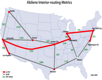
We’ll look at data traffic on the Abilene network:
Source: Internet2, circa 2005
Each row is a 10-minute interval over one week (1008 rows); each column is one origin–destination flow between two of the eleven Abilene routers (121 columns).
import os, urllib.requestdef data_file(path):"""Course data file: use a local copy (here, or in the repo root above a notebook in jupyter_notebooks/), else fetch it from the Materials repo (Colab)."""for prefix in ('', '../'):if os.path.exists(prefix + path):return prefix + path os.makedirs(os.path.dirname(path) or'.', exist_ok=True) urllib.request.urlretrieve('https://raw.githubusercontent.com/tools4ds/DS701-Materials-FA26/main/'+ path, path)return pathimport pandas as pdwithopen(data_file('data/net-traffic/AbileneFlows/odnames'),'r') as f: odnames = [line.strip() for line in f]dates = pd.date_range('9/1/2003', freq ='10min', periods =1008)Atraf = pd.read_table(data_file('data/net-traffic/AbileneFlows/X'), sep=' ', header=None, names=odnames, engine='python')Atraf.index = datesAtraf.shape
(1008, 121)
Code
Atraf.iloc[:4, :6]
ATLA-ATLA
ATLA-CHIN
ATLA-DNVR
ATLA-HSTN
ATLA-IPLS
ATLA-KSCY
2003-09-01 00:00:00
8466132.0
29346537.0
15792104.0
3646187.0
21756443.0
10792818.0
2003-09-01 00:10:00
20524567.0
28726106.0
8030109.0
4175817.0
24497174.0
8623734.0
2003-09-01 00:20:00
12864863.0
27630217.0
7417228.0
5337471.0
23254392.0
7882377.0
2003-09-01 00:30:00
10856263.0
32243146.0
7136130.0
3695059.0
28747761.0
9102603.0
As we would expect, our traffic matrix has rank 121:
np.linalg.matrix_rank(Atraf)
np.int64(121)
However – perhaps it has low effective rank.
The numpy routine for computing the SVD is np.linalg.svd. We ask for the thin SVD:
u, s, vt = np.linalg.svd(Atraf, full_matrices=False)u.shape, s.shape, vt.shape
((1008, 121), (121,), (121, 121))
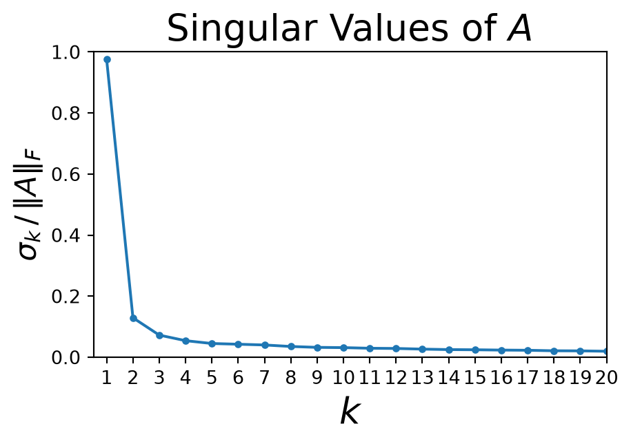
Now let’s look at the singular values of Atraf to see if it can be usefully approximated as a low-rank matrix:
This classic, sharp-elbow tells us that a few singular values are very large, and most singular values are quite small. In fact \(\sigma_1^2\) alone is 95% of \(\sum_i\sigma_i^2 = \Vert A\Vert_F^2\).
Zooming in for just small \(k\) values, and scaling by \(\Vert A\Vert_F\), we can see that the elbow is around 4 - 6 singular values:
Why should a week of traffic on 121 links be described so well by 20 patterns?
A model is a description of the data that is simpler than the data, and modeling works surprisingly often. William of Ockham (c. 1300) put it this way:
Entities must not be multiplied beyond necessity.
that is, among competing hypotheses, prefer the one with the fewest assumptions.
“Occam’s razor” is an observation about the world: it is more common for a set of observations to be generated by a simple process than a complex one. The world is full of simple, but often hidden, patterns — and low effective rank is one precise, measurable form of that simplicity.
Low Effective Rank is Common
In practice many datasets have low effective rank.
We consider the following examples:
Likes on Facebook, Yelp reviews and Tweets (the site formerly known as Twitter),
User preferences over time,
Images.
Social Media Activity
Here, the matrices are Users \(\times\) Categories:
Number of Facebook likes: Users \(\times\) Page Categories
Number of Yelp reviews: Users \(\times\) Yelp Categories
Number of Tweets: Users \(\times\) Topic Categories
Source: [Viswanath et al., Usenix Security, 2014]
“Fraction of variance” of component \(i\) is \(\sigma_i^2/\sum_j\sigma_j^2\) of the centered matrix — that is PCA (next lecture), but the same elbow. The paper’s user \(\times\) time-bin matrices are not low rank: common, not universal.
Netflix
Example: the Netflix prize worked with partially-observed (sparse) rating matrices like this:
where the rows correspond to users, the columns to movies, and the entries are ratings.
Although the problem matrix was of size 500,000 \(\times\) 18,000, the winning approach modeled the matrix as having rank 20 to 40.
Source: [Koren et al, IEEE Computer, 2009]
Not quite the SVD
The Netflix matrix is about 99% empty, and the SVD needs every entry. The winning entry instead used matrix factorization: a rank-\(k\) model \(\tilde U\tilde V\) fitted only to the observed ratings. Same low-rank idea, different algorithm — it is the second half of Lecture 19.
Images
Image data often shows low effective rank.
For example, here is an original \(512 \times 512\) photo:
Code
boat = np.loadtxt(data_file('data/images/boat/boat.dat'))import matplotlib.cm as cmplt.figure()plt.imshow(boat, cmap=cm.Greys_r)plt.axis('off')plt.show()
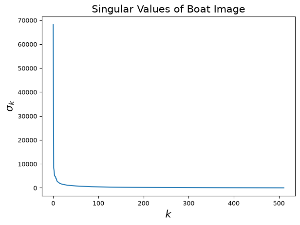
Treat the image as a matrix and then compute the singular values. They span five orders of magnitude, so we use a log scale:
Code
u, s, vt = np.linalg.svd(boat, full_matrices=False)plt.semilogy(range(1, 1+len(s)), s)plt.xlabel('$k$', size=16)plt.ylabel(r'$\sigma_k$(log scale)', size=16)plt.title('Singular Values of Boat Image', size=16)plt.show()
This image is 512 \(\times\) 512. As a matrix, it has rank of 512.
But its effective rank is low: \(\sigma_1\) is eight times \(\sigma_2\), and by \(k = 40\) the singular values are down to about 1% of \(\sigma_1\).
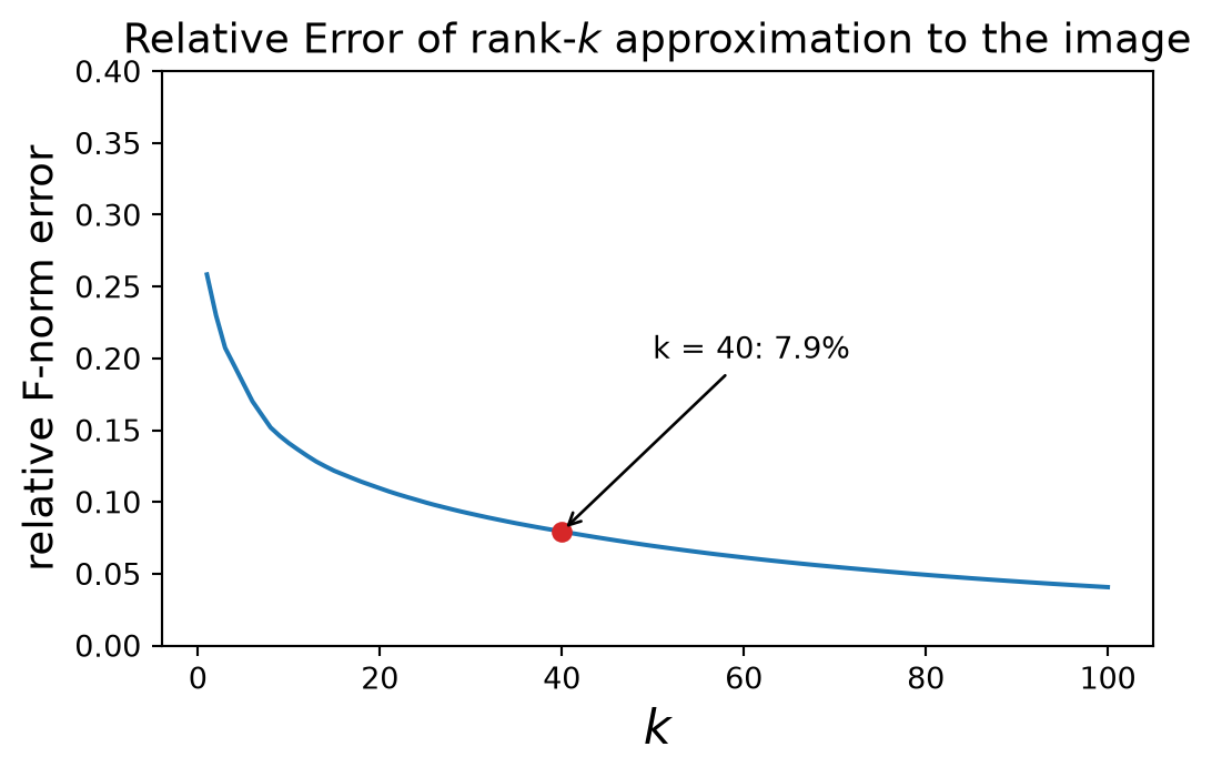
The Eckart–Young formula turns that into an error curve:
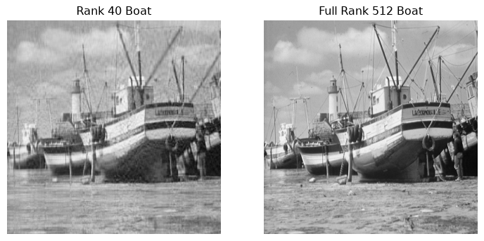
At rank 40 the relative error is 7.9%, and we store \(k(m + n + 1) = 40\cdot(512 + 512 + 1) = 41{,}000\) numbers instead of \(512^2 = 262{,}144\) — a \(6.4\times\) compression.
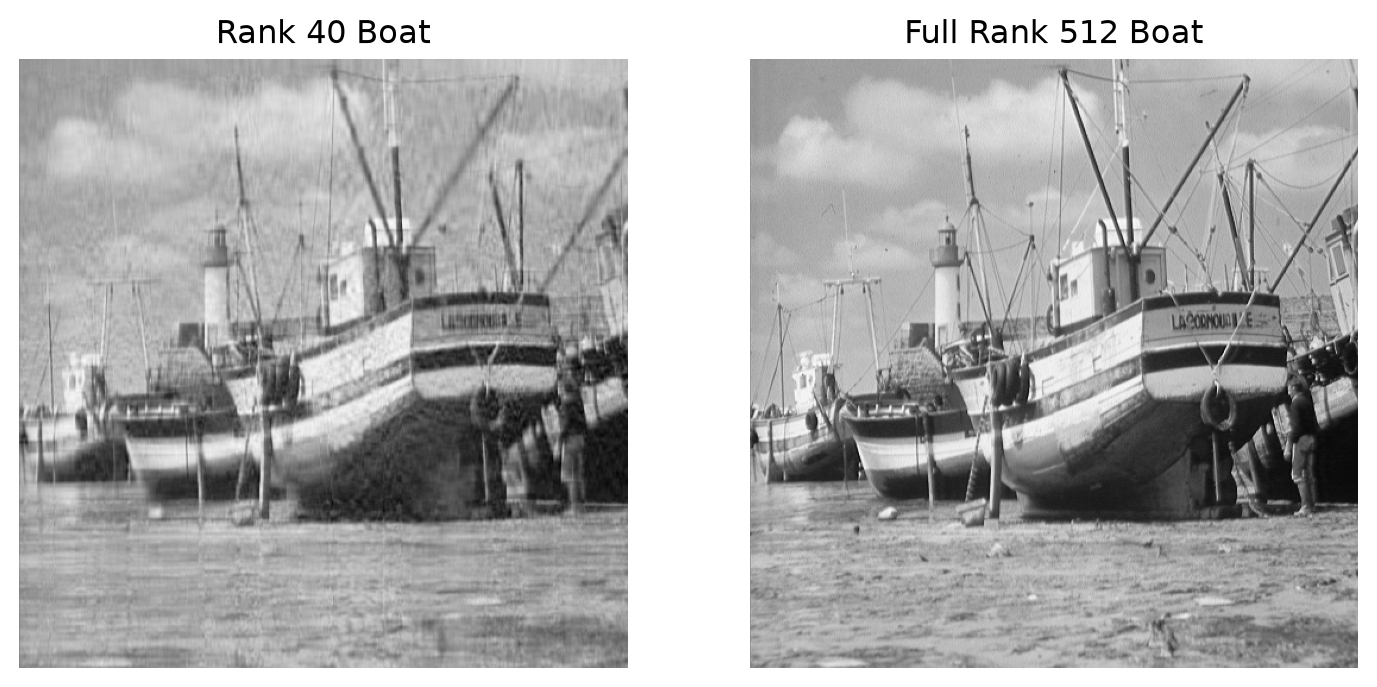
Let’s find the closest rank-40 matrix and view it.
k =40boatApprox = u[:, :k] @ np.diag(s[:k]) @ vt[:k]
How can we understand the low-effective-rank phenomenon in general?
There are two helpful interpretations:
Common Patterns
Latent Factors
Low Rank Implies Common Patterns
The first interpretation of low-rank behavior is in answering the question:
“What is the strongest pattern in the data?”
Remember that using the SVD we form the low-rank approximation as
\[ A^{(k)} = U'\Sigma'(V')^T\]
and
\(U'\) are the \(k\) leftmost columns of \(U\),
\(\Sigma'\) is the \(k\times k\) upper left submatrix of \(\Sigma\), and
\(V'\) are the \(k\) leftmost columns of \(V\).
In this interpretation, we think of each column of \(A^{(k)}\) as a combination of the columns of \(U'\).
How can this be helpful?
Common Patterns: Traffic Example
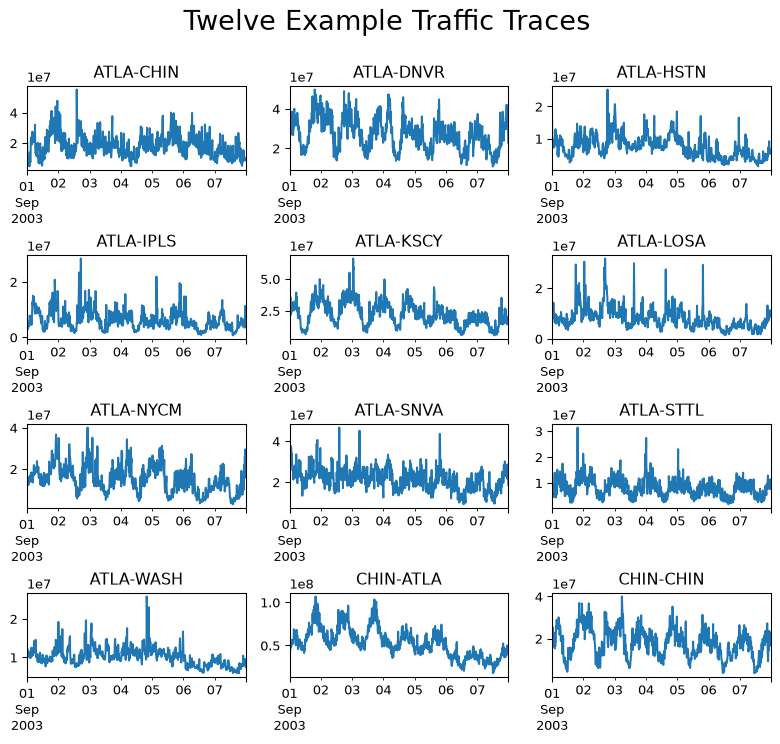
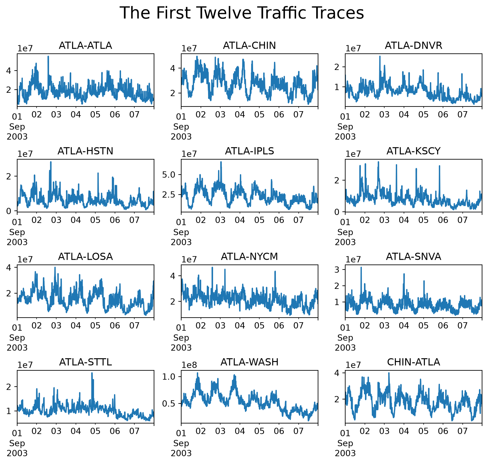
Consider the set of traffic traces. There are clearly some common patterns. How can we find them?
Code
plt.figure(figsize=(10, 8))for i inrange(12): ax = plt.subplot(4, 3, i +1) Atraf.iloc[:, i].plot() plt.title(odnames[i])plt.subplots_adjust(hspace=1)plt.suptitle('The First Twelve Traffic Traces', size=20)plt.show()
Let’s use as our example the ATLA-CHIN flow — traffic from Atlanta to Chicago. It is the second column of \(A\) (the first, ATLA-ATLA, is traffic that enters and leaves at Atlanta):
j = odnames.index('ATLA-CHIN')j
1
The outer-product form of the SVD tells us that column \(j\) is
where \(v_{ij}\) is the \(j\)-th entry of \(\mathbf{v}_i\) — so the coefficients are the \(j\)-th column of \(V^T\).
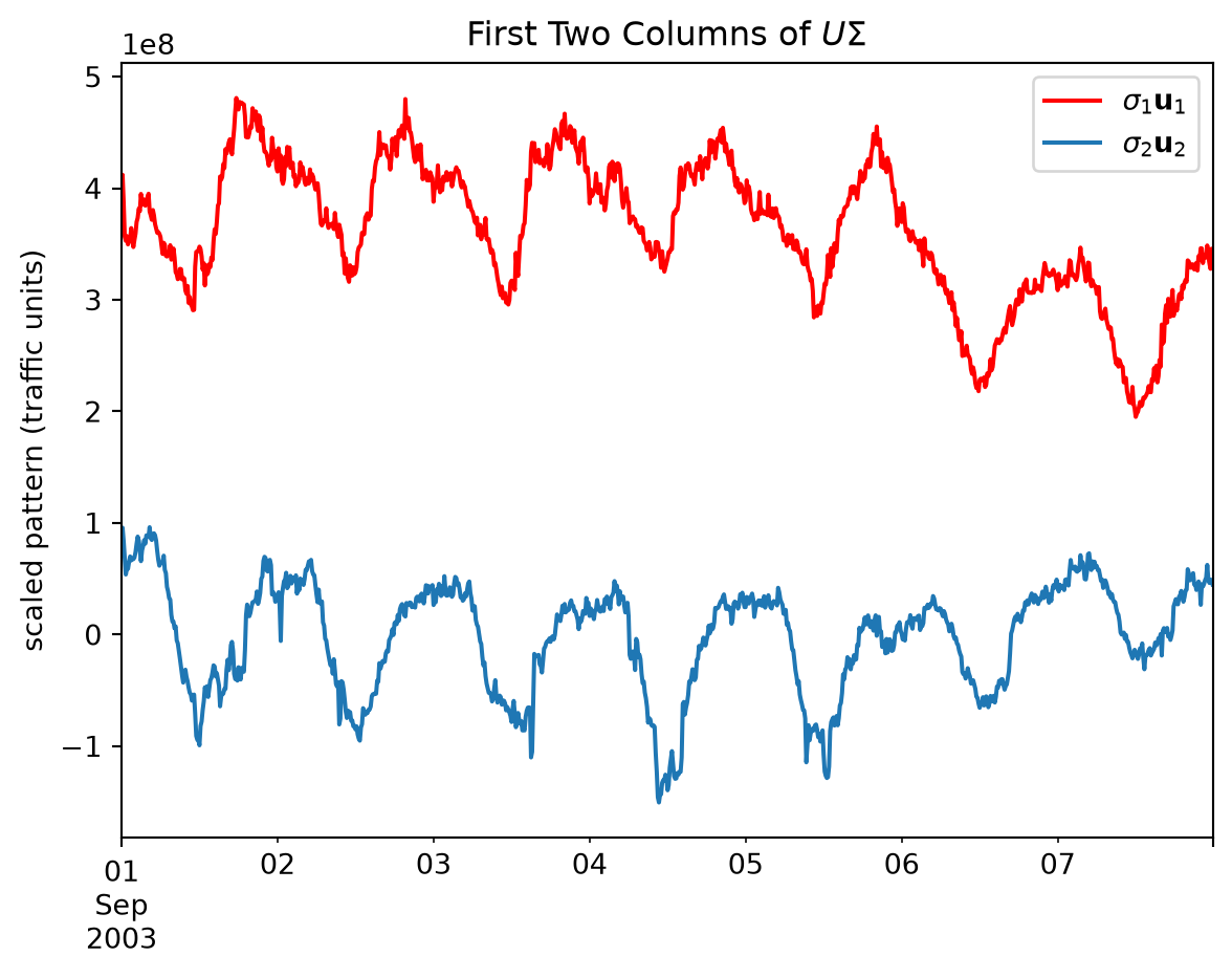
Every one of the 121 traces is a combination of the same\(k\) vectors \(\mathbf{u}_1, \ldots, \mathbf{u}_k\); only the coefficients change from trace to trace. In other words, \(\mathbf{u}_1\) (the first column of \(U\)) is the “strongest” pattern occurring in \(A\), and its strength is measured by \(\sigma_1\).
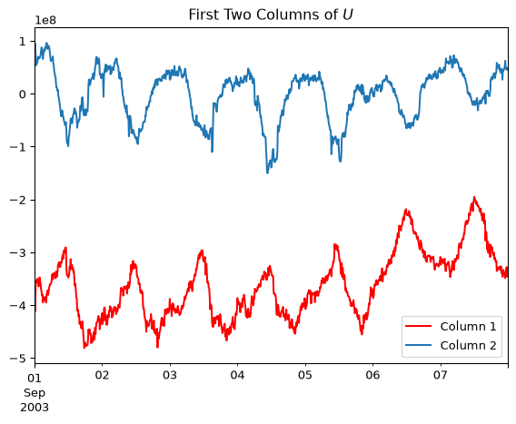
Here is a view of the first 2 columns of \(U\Sigma\), i.e. \(\sigma_1\mathbf{u}_1\) and \(\sigma_2\mathbf{u}_2\), for the traffic matrix data.
These are the strongest patterns occurring across all of the 121 traces.
Code
u, s, vt = np.linalg.svd(Atraf, full_matrices=False)# Singular vectors are only determined up to sign, and LAPACK happened to# return u_1 entirely negative. Flip u_1 and v_1 together (which leaves# sigma_1 u_1 v_1^T unchanged) so the pattern reads as traffic volume.sign = np.sign(u[:, 0].sum())u[:, 0] *= signvt[0] *= signuframe = pd.DataFrame(u @ np.diag(s), index=dates)uframe[0].plot(color='r', label=r'$\sigma_1 \mathbf{u}_1$')uframe[1].plot(label=r'$\sigma_2 \mathbf{u}_2$')plt.legend(loc='best')plt.ylabel('scaled pattern (traffic units)')plt.title(r'First Two Columns of $U\Sigma$')plt.show()
The first pattern is the daily rhythm shared by every flow: low overnight, high during the day, weaker at the weekend. Each trace, ATLA-CHIN included, is mostly a rescaled copy of it — which is exactly what \(\sigma_1^2\) being 95% of \(\Vert A\Vert_F^2\) means.
Low Rank Defines Latent Factors
The next interpretation of low-rank behavior is that it exposes “latent factors” that describe the data.
In this interpretation, we think of each element of \(A^{(k)}=U'\Sigma'(V')^T\) as the inner product of a row of \(U'\Sigma'\) and a column of \((V')^{T}\) (equivalently a row of \(V'\)).
Let’s say we are working with a matrix of users and items.
In particular, let the items be movies and matrix entries be ratings, as in the Netflix prize.
where the rows of \(A\) are the users and the columns are movie ratings.
Then the rating that a user gives a movie is the inner product of a \(k\)-element vector that corresponds to the user, and a \(k\)-element vector that corresponds to the movie.
We can think of user \(i\)’s preferences as being captured by row \(i\) of \(\tilde{U}\), which is a point in \(\mathbb{R}^k\).
We have described everything we need to know to predict user \(i\)’s ratings via a \(k\)-element vector.
The \(k\)-element vector is called a latent factor.
Likewise, we can think of column \(j\) of \(\tilde{V}\) as a “description” of movie \(j\) (another latent factor).
The value in using latent factors comes from the summarization of user preferences, and the predictive power one obtains.
For example, the winning entry in the Netflix prize competition modeled user preferences with 20 latent factors.
The remarkable thing is that a person’s preferences for all 18,000 movies can be reasonably well captured in a vector of dimension 20!
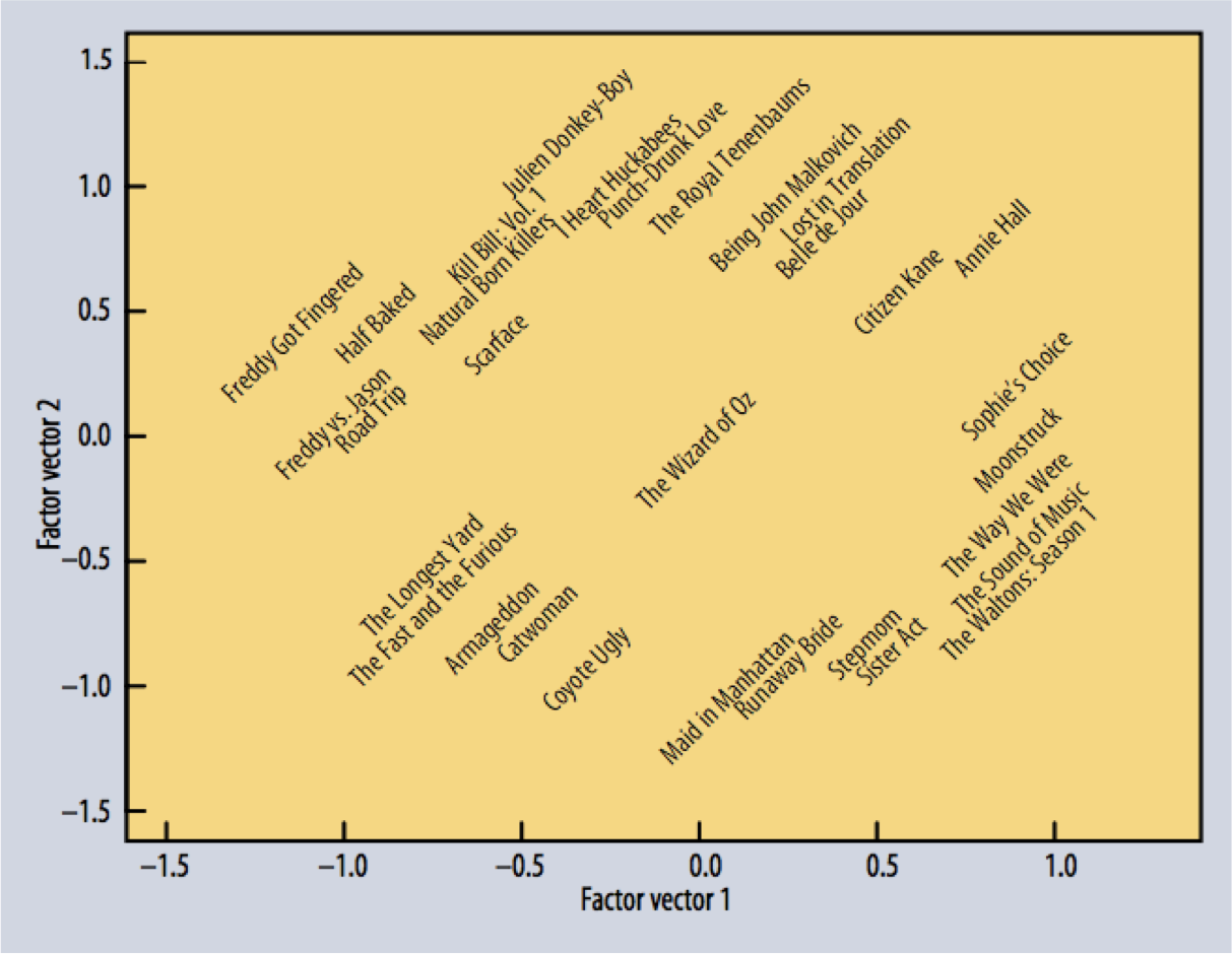
Here is a figure from the paper that described the winning strategy in the Netflix prize.
It shows a hypothetical latent space in which each user, and each movie, is represented by a latent vector.
Source: Koren et al, IEEE Computer, 2009
In practice, this is perhaps a 20- or 40-dimensional space.
Here are some representations of movies in that space (reduced to 2-D).
Notice how the space seems to capture similarity among movies!
Source: Koren et al, IEEE Computer, 2009
Summary
The SVD \(A = U\Sigma V^T\) exists for every matrix: the \(\mathbf{v}_i\) are the eigenvectors of the symmetric matrix \(A^TA\), \(\sigma_i^2\) are its eigenvalues, and \(\mathbf{u}_i = A\mathbf{v}_i/\sigma_i\).
When we are working with data matrices, it is valuable to consider the effective rank.
Many (many) datasets in real life show low effective rank.
This property can be explored precisely using the Singular Value Decomposition of the matrix: by the Eckart–Young theorem, the truncated SVD is the best rank-\(k\) approximation, and its error is the sum of the discarded \(\sigma_i^2\).
When low effective rank is present
the matrix can be compressed with only small loss of accuracy,
we can extract the strongest patterns in the data,
we can describe each data item in terms of the inner product of latent factors.
Next lecture: center the columns of a data matrix and take its SVD. The columns of \(V\) are the principal directions and \(\sigma_i^2/(m-1)\) is the variance along each — the \(A^TA = V\Sigma^2V^T\) identity above is PCA.


Social Media Activity
Here, the matrices are Users \(\times\) Categories:
Source: [Viswanath et al., Usenix Security, 2014]
“Fraction of variance” of component \(i\) is \(\sigma_i^2/\sum_j\sigma_j^2\) of the centered matrix — that is PCA (next lecture), but the same elbow. The paper’s user \(\times\) time-bin matrices are not low rank: common, not universal.