Recap: Causal Inference I

DS701 Session 16 — Wed Oct 28, 2026

Today’s plan

• 5 min — knowledge-check review
• 20 min — highlights and Q&A (answer or pass — answering always earns credit)
• 60 min — in-class activity (small groups)
• wrap-up and cold-call check-ins

Quiz 2 is five days away (Mon Nov 2) and covers sessions 9–15 — not today. Causal inference (this lecture and lecture 15) is examined on quiz 3. Today is not quiz review; use office hours for that.

Knowledge-Check Review

KC 1: Two readings of one coefficient

A regression coefficient \(\hat\beta_1\) on \(X\) has two possible readings — an associational one and a causal one. State both in one sentence each, say which one least squares always gives you, and give the definition of a confounder from the lecture.

KC 2: The selection-bias term

The lecture decomposed the naive difference in means, \(\mathbb{E}[Y \mid T{=}1] - \mathbb{E}[Y \mid T{=}0]\), into a causal part plus a selection-bias term. In words, what does the selection-bias term measure, why is it nonzero in the hospital-visits example, and why does randomly assigning \(T\) make it zero?

KC 3: Kidney stones, then ice cream

In the kidney-stone study, Treatment A had the higher recovery rate for small stones and for large stones, yet Treatment B had the higher rate overall. Which comparison should a doctor trust, and why? Then connect it to the ice cream regression: what plays the role of stone size there, and what did “adjusting for it” look like in code?

Highlights

1. A regression coefficient is an association, not an effect

A regression coefficient is an association, not an effect. OLS estimates \(P(Y \mid X)\); a causal claim is about \(P(Y \mid do(X))\), and the two differ whenever there is confounding.

Prediction — seeing

\[ P(Y \mid X = x) \]

“Among people I observe with \(X = x\), what is \(Y\)?”

Every model in this course so far. Rung 1 of Pearl’s ladder.

Intervention — doing

\[ P(Y \mid do(X = x)) \]

“If I set \(X = x\) for everyone, what is \(Y\)?”

What a decision-maker needs. Rung 2.

The hospital model is a good predictor (“I see a visit, I predict higher mortality”) and a catastrophic guide to action (“close the hospitals”). Same table, two readings — the whole subject of these two lectures is the gap between them.

2. A confounder is a common cause

A confounder is a common cause of treatment and outcome. Adjusting for it (holding it fixed, or adding it to the regression) removes the spurious association — but only if you measured it and knew to include it.

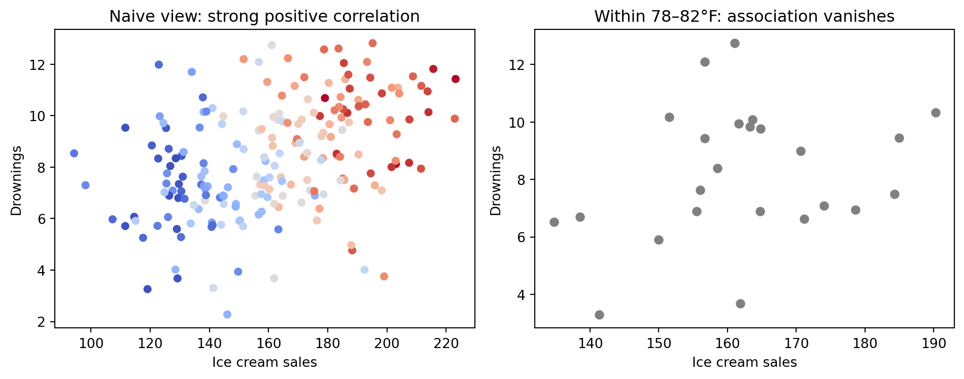
• drownings ~ ice_cream: slope \(+0.032\), \(p \approx 0\) — every Lecture 11 diagnostic happy. Truth: zero (ice cream is not in the equation for drownings).
• drownings ~ ice_cream + temp: slope \(-0.007\). Adding the confounder = looking within a temperature band (right panel).
• Which variables to add is a causal question the fitting procedure cannot answer. Unmeasured temperature → no model selection saves you.

3. Potential outcomes define the effect — you observe one

Potential outcomes \(Y(1), Y(0)\) define the effect; you only ever observe one. This is the fundamental problem of causal inference, so we estimate averages like the \(\text{ATE} = \mathbb{E}[Y(1) - Y(0)]\).

Unit	\(T_i\)	\(Y_i(0)\)	\(Y_i(1)\)	\(\tau_i\)
Ann	1	?	7	?
Bob	0	4	?	?
Cara	1	?	9	?
Dan	0	3	?	?

\(Y_i^{\text{obs}} = T_i\, Y_i(1) + (1 - T_i)\, Y_i(0)\)

• \(\tau_i = Y_i(1) - Y_i(0)\) needs both columns — the counterfactual is missing. Causal inference is a missing-data problem.
• So target averages: \(\text{ATE} = \mathbb{E}[Y(1)] - \mathbb{E}[Y(0)]\); ATT \(= \mathbb{E}[Y(1) - Y(0) \mid T{=}1]\); CATE \(= \mathbb{E}[Y(1) - Y(0) \mid X{=}x]\).
• The tempting estimator is the column means we can see: \(\mathbb{E}[Y \mid T{=}1] - \mathbb{E}[Y \mid T{=}0]\) — next slide says what that actually is.

4. Naive difference \(=\) causal effect \(+\) selection bias

Naive difference in means \(=\) causal effect \(+\) selection bias. Simpson’s paradox is what selection bias looks like in a table: within-group and overall comparisons can point in opposite directions.

\[ \underbrace{\mathbb{E}[Y(1)\mid T{=}1] - \mathbb{E}[Y(0)\mid T{=}0]}_{\text{naive difference}} = \underbrace{\text{ATT}}_{\text{causal}} + \underbrace{\mathbb{E}[Y(0)\mid T{=}1] - \mathbb{E}[Y(0)\mid T{=}0]}_{\text{selection bias}} \]

	Treatment A (surgery)	Treatment B (less invasive)
Small stones	81/87 = 93%	234/270 = 87%
Large stones	192/263 = 73%	55/80 = 69%
Overall	273/350 = 78%	289/350 = 83%

• A wins in every stratum; B wins overall — because A got 263 of its 350 patients from the hard stratum. Case-mix, not effect.
• The coefficient on T in Y ~ T is the naive difference. It inherits the same bias.

5. Randomization zeroes the bias term

Randomization makes treatment independent of potential outcomes, so the selection-bias term is zero and the naive difference is unbiased for the ATE.

\[ \{Y_i(0), Y_i(1)\} \perp\!\!\!\perp T_i \]

• Coin flip ⇒ treated and untreated groups identical in expectation — on every trait, measured or not.
• \(\mathbb{E}[Y(0)\mid T{=}1] = \mathbb{E}[Y(0)\mid T{=}0]\) ⇒ bias term \(=0\).
• No list of confounders needed. That is why an A/B test is the gold standard.

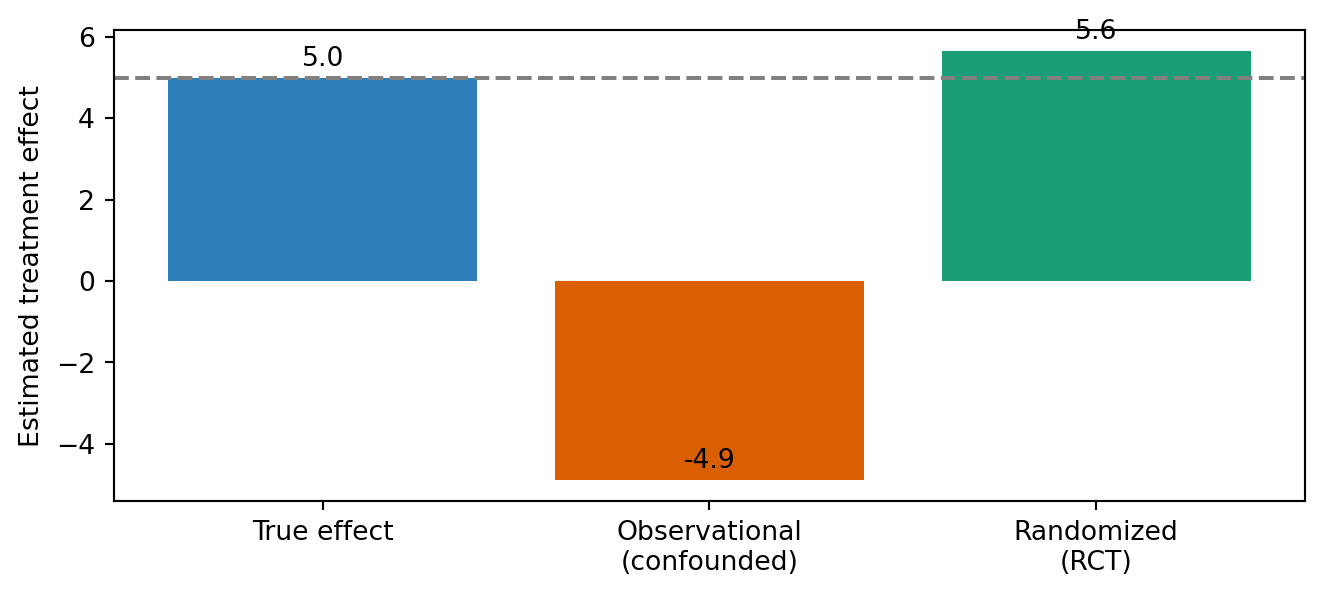
True effect \(+5\); sicker patients likelier to be treated ⇒ observational \(-4.9\); coin flip ⇒ \(+5.6\).

When you can randomize, do. When you cannot — cost, ethics, the treatment already happened — you must decide what to adjust for. Today’s activity ends by showing you that adjusting for the wrong variable can create bias from nothing. That is where Lecture 15 begins.

In-Class Activity

Activity: confounding scenarios, then watch regression lie

Goal: classify real-world comparisons (confounded / reverse / Simpson / randomized) and name the confounder; recompute a Simpson’s-paradox table by hand and adjust it; then simulate a confounder with a known true effect \(\beta\), watch Y ~ X get it wrong, Y ~ X + Z recover it, and randomization make the naive fit right — and finally condition on a collider and watch a spurious effect appear from nothing.

• Work in groups of 2–3. Open your section’s notebook (different scenarios, table, and \(\beta\)).
• Parts marked (autograded) are submitted to Gradescope; the rest is participation.
• Staff will circulate — be ready to explain any part of your work.
• Dependencies: numpy, pandas, matplotlib, statsmodels.

Section A1

Section B1

The activity notebook goes live on the day of the lecture. Colab is optional — you can also open it on GitHub and run it locally.

Going deeper

Full lecture notes: Causal Inference I: Correlation, Causation, and Counterfactuals

• What does a coefficient mean? — the two readings, side by side
• A regression you would recognize — the ice cream / drowning fit and its data-generating code
• Confounding — definition; adjusting by adding temp
• Two different questions — \(P(Y \mid X)\) vs. \(P(Y \mid do(X))\); the ladder of causation
• Where do spurious associations come from? — the five sources
• The potential outcomes framework, the fundamental problem, the ATE
• Selection bias — the decomposition of the naive difference
• Kidney stones and Berkeley admissions — Simpson’s paradox in real tables
• The gold standard: randomized experiments — independence kills the bias term; the simulated drug study
• Next: Causal Inference II — causal graphs, what to adjust for and what not to