Recap: Causal Graphs and Estimating Effects
DS701 Session 18 — Wed Nov 4, 2026
The graph is your assumptions, not the data’s
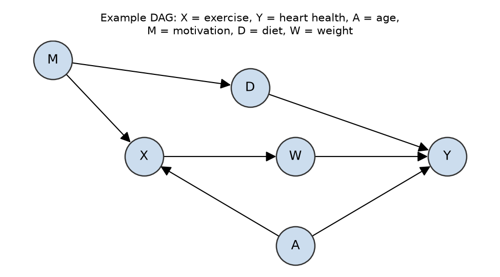
- Node = variable; arrow \(A \to X\) = “\(A\) is a direct cause of \(X\)” (\(A\) parent, \(X\) child).
- Directed path = follow the arrows: \(X \to W \to Y\). Nodes reachable this way are \(X\)’s descendants (\(W, Y\)).
- Acyclic: nothing is its own ancestor — cause precedes effect. Hence DAG.
- Path (undirected) = any chain of arrows, direction ignored: \(X \leftarrow A \to Y\) counts too.
Effects flow along directed paths; spurious association along the others. Domain knowledge draws the graph — data cannot — but once drawn, it tells you exactly what to control for.
Every path is chains, forks and colliders
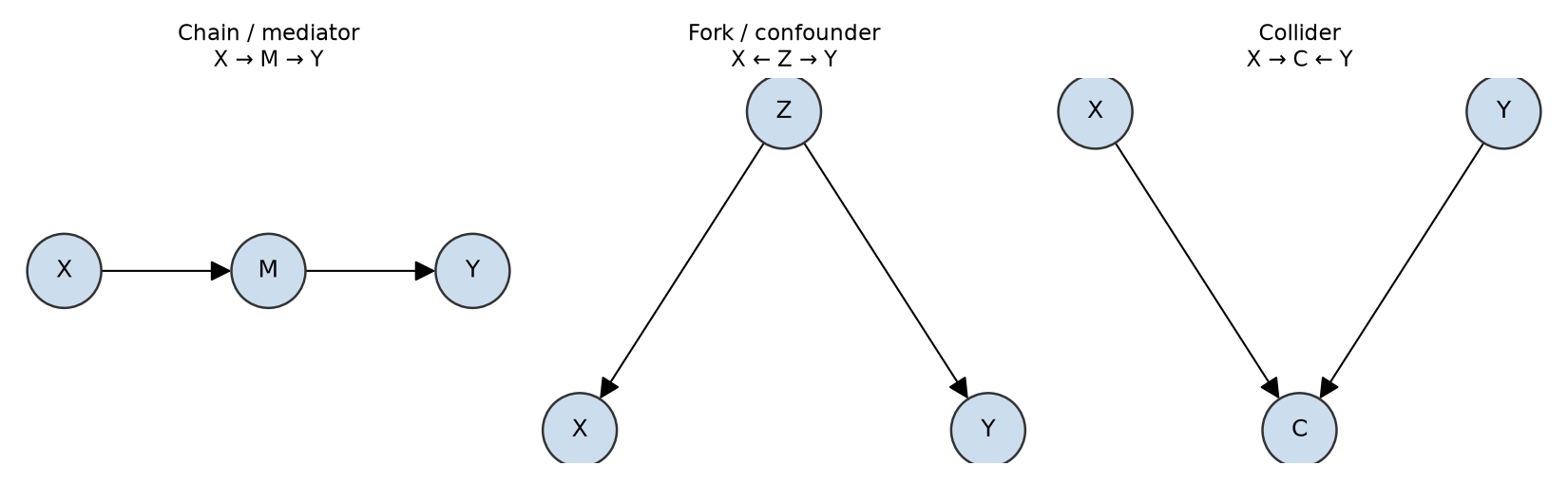
- Chain / fork node: open by default, blocked if you condition on it (adjust, stratify, put it in the regression).
- Collider node: blocked by default, opened if you condition on it — or on any of its descendants.
A path is blocked if at least one interior node is blocked; \(X\) and \(Y\) are independent given \(S\) when every path between them is blocked. Sanity check: \(X \leftarrow A \to Y\) is open (fork) — the ice-cream/temperature confounding of Lecture I; condition on \(A\) and it closes.
Worked example, five steps
\(A \to X,\ A \to Y,\ M \to X,\ M \to D,\ D \to Y,\ X \to W,\ W \to Y\)
- Paths: \(X \to W \to Y\); \(X \leftarrow A \to Y\); \(X \leftarrow M \to D \to Y\).
- Causal: \(X \to W \to Y\) — leave \(W\) alone.
- Backdoors: \(X \leftarrow A \to Y\) open (fork at \(A\)); \(X \leftarrow M \to D \to Y\) open (fork at \(M\), chain at \(D\)). No colliders.
- Block the first with \(A\); the second with \(M\) or \(D\).
- Valid: \(\{A, M\}\), \(\{A, D\}\), \(\{A, M, D\}\). Not \(\{A\}\) (backdoor left open); not anything with \(W\) (descendant of \(X\)).
Y ~ X + A + M recovers the total effect; Y ~ X + A + M + W does not.
After identification: the estimator is the easy part
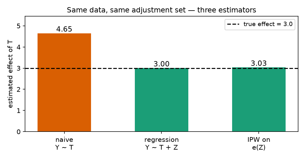
Lecture simulation: \(Y = 3T + 2Z + \varepsilon\), sicker (\(Z\)) more likely treated.
Given a valid \(S\) (ignorability), any of these recovers the effect:
- Regression — include \(S\) as covariates, read the coefficient on \(T\).
- Stratification — effect within strata of \(S\), averaged with population weights (the kidney-stone table).
- Matching on \(S\).
- Propensity score \(e(S) = P(T{=}1 \mid S)\) — match or weight (IPW: \(1/e\) treated, \(1/(1-e)\) control) to build a pseudo-population where \(T \perp S\).
Same \(S\), same answer. A wrong \(S\) gives a wrong answer with a tight standard error — the estimator cannot rescue a bad graph.
Activity: backdoor identification by hand, then watch a wrong adjustment set lie
Goal: on five DAGs (drawn with networkx), list every backdoor path, mark it open or blocked, code the two rules into a checker, and propose one valid and one invalid adjustment set per DAG. Then simulate data from one of those DAGs with a known effect and estimate it four ways — naive, correct set, wrong set (mediator / collider), inverse-propensity weighting — and see which ones recover the truth.
- Work in groups of 2–3. Open your section’s notebook — the DAG subset and the simulated effect differ by section.
- Parts marked (autograded) are submitted to Gradescope; the rest is participation.
- Staff will circulate — be ready to explain any part of your work.
- Dependencies:
numpy,pandas,matplotlib,networkx,statsmodels,scikit-learn.
Section A1 

Section B1
The activity notebook goes live on the day of the lecture. Colab is optional — you can also open it on GitHub and run it locally.