Neural Networks II: Making Training Work

Introduction

Code
import warnings
import numpy as np
import matplotlib.pyplot as plt
import pandas as pd
from sklearn.exceptions import ConvergenceWarning
from slideUtilities import OKABE_ITO

%matplotlib inline

Last time (Neural Networks I) was about how learning works. Today is deliberately practical: making training work with scikit-learn.

We’ll cover:

  • MLPClassifier and MLPRegressor
  • A classification example (MNIST) and a regression example (California housing)
  • Hyperparameter tuning with grid search
  • Diagnosing training from its curves: an unscaled fit, three learning rates, and a network that overfits on purpose
  • Repairing what the curves show, and what scikit-learn’s MLP cannot do

Last Time: How Learning Works

  • Model: an MLP is layers of neurons, \(\mathbf{h}_{k+1} = f(\boldsymbol{\beta}_k + \boldsymbol{\Omega}_k \mathbf{h}_k)\), with a non-linear activation \(f\) (e.g. ReLU)
  • Loss: MSE for regression, cross-entropy for classification; training means minimizing it over the parameters \(\theta\)
  • Gradient descent: \(\theta \leftarrow \theta - \eta \nabla_\theta L\), with learning rate \(\eta\)
  • Backpropagation: the chain rule run backwards over the compute graph gives every \(\partial L / \partial \theta\) at about the cost of one forward pass
  • Stochastic / mini-batch GD: estimate the gradient from a small batch of samples per step

Today: The Knobs

Every one of those ideas shows up as an argument you have to choose:

Concept scikit-learn argument
Layers and neurons hidden_layer_sizes
Activation \(f\) activation
Learning rate \(\eta\) learning_rate_init, learning_rate\(^*\)
Mini-batch size batch_size
Optimizer solver ('adam', 'sgd', 'lbfgs')
Epochs / stopping max_iter, early_stopping, n_iter_no_change
Regularization alpha

\(^*\) learning_rate is a schedule ('constant', 'invscaling', 'adaptive') and is used by solver='sgd' only; adam adapts its step sizes on its own.

The rest of the lecture is about setting these sensibly – and what goes wrong when you don’t.

Neural Networks in Scikit-Learn

MLPClassifier and MLPRegressor

Scikit-learn provides simple, high-level interfaces:

  • MLPClassifier: Multi-layer Perceptron classifier
  • MLPRegressor: Multi-layer Perceptron regressor

Key features:

  • Multiple hidden layers with various activation functions
  • Multiple solvers: 'adam', 'sgd', 'lbfgs'
  • Built-in regularization (L2 penalty)
  • Early stopping support
  • Easy integration with scikit-learn pipelines

Architecture Specification

Specify architecture as a tuple:

# Single hidden layer with 100 neurons
hidden_layer_sizes=(100,)

# Two hidden layers: 100 and 50 neurons
hidden_layer_sizes=(100, 50)

# Three hidden layers
hidden_layer_sizes=(128, 64, 32)

Input and output layers are automatically determined from your data!

Scikit-Learn vs PyTorch/TensorFlow


Use Scikit-Learn for:

  • Small to medium datasets (< 100K samples)
  • Standard feedforward architectures
  • Rapid prototyping needed
  • Integration with scikit-learn pipelines
  • CPU training is sufficient

Use PT/TF for:

  • Large datasets (> 100K samples)
  • Complex architectures (CNNs, RNNs)
  • GPU acceleration required
  • Production deployment
  • Research and experimentation

Classification Example: MNIST

Load the MNIST Dataset

Let’s classify handwritten digits (0-9):

from sklearn.datasets import fetch_openml
from sklearn.model_selection import train_test_split

# Load MNIST data
print("Loading MNIST dataset...")
X, y = fetch_openml('mnist_784', version=1, return_X_y=True,
                    as_frame=False, parser='auto')

# Convert labels to integers
y = y.astype(int)

# Use subset for faster demo
X, _, y, _ = train_test_split(X, y, train_size=10000,
                               stratify=y, random_state=42)

print(f"Dataset shape: {X.shape}")
print(f"Number of classes: {len(np.unique(y))}")
Loading MNIST dataset...
Dataset shape: (10000, 784)
Number of classes: 10

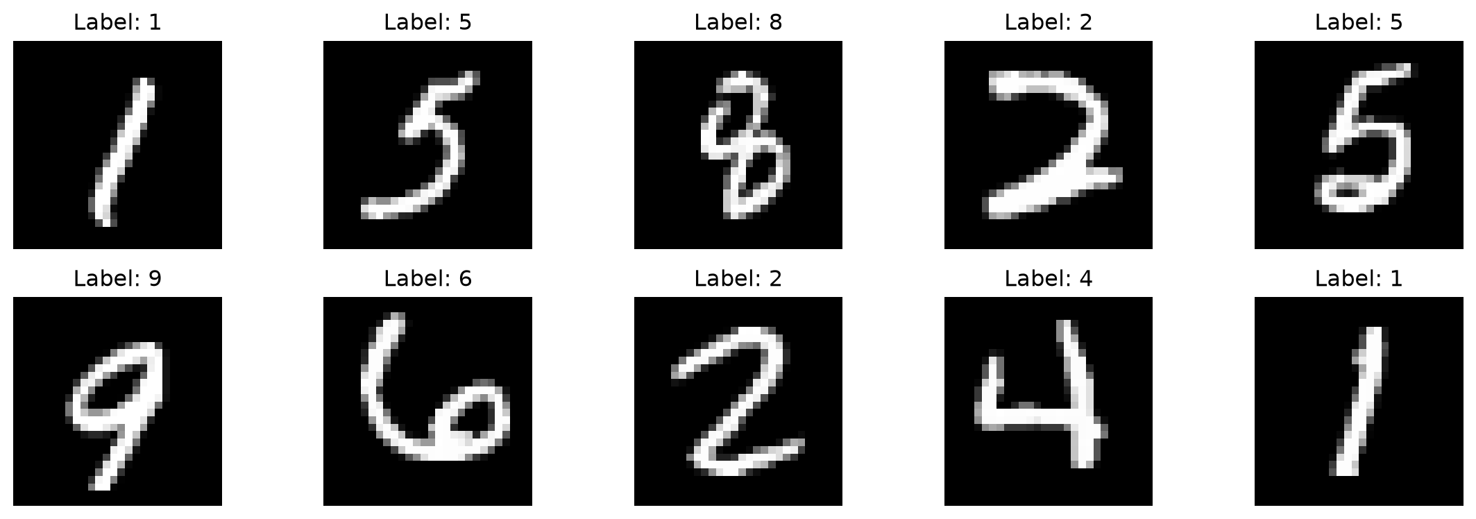
Visualize the Data

Code
fig, axes = plt.subplots(2, 5, figsize=(12, 4))
for i, ax in enumerate(axes.flat):
    ax.imshow(X[i].reshape(28, 28), cmap='gray')
    ax.set_title(f'Label: {y[i]}')
    ax.axis('off')
plt.tight_layout()
plt.show()

Each image is 28×28 pixels = 784 features

Prepare the Data

# Split into training and test sets
X_train, X_test, y_train, y_test = train_test_split(
    X, y, test_size=0.2, random_state=42
)

# Scale features to [0, 1]
X_train_scaled = X_train / 255.0
X_test_scaled = X_test / 255.0

print(f"Training set: {X_train.shape[0]} samples")
print(f"Test set: {X_test.shape[0]} samples")
print(f"Feature range: [{X_train_scaled.min():.2f}, {X_train_scaled.max():.2f}]")
Training set: 8000 samples
Test set: 2000 samples
Feature range: [0.00, 1.00]

Important

Always scale/normalize your features for neural networks! This helps gradient descent converge faster. We will see what happens when you don’t in Why Scaling Matters.

Create the MLP

from sklearn.neural_network import MLPClassifier

# Create MLP with 2 hidden layers
mlp = MLPClassifier(
    hidden_layer_sizes=(128, 64),  # Architecture
    activation='relu',              # Activation function
    solver='adam',                  # Optimizer (uses mini-batches)
    alpha=0.0001,                   # L2 regularization
    batch_size=64,                  # Mini-batch size
    learning_rate_init=0.001,       # Initial learning rate
    max_iter=20,                    # Number of epochs
    random_state=42,
)

verbose=True would print the training loss after every epoch; the curve on the next slide shows the same numbers.

Train the model

mlp.fit(X_train_scaled, y_train)
print(f"Epochs run: {mlp.n_iter_} of max_iter={mlp.max_iter}")
print(f"Training loss, last three epochs: {np.round(mlp.loss_curve_[-3:], 4)}")
Epochs run: 20 of max_iter=20
Training loss, last three epochs: [0.0034 0.0028 0.0025]

Warning

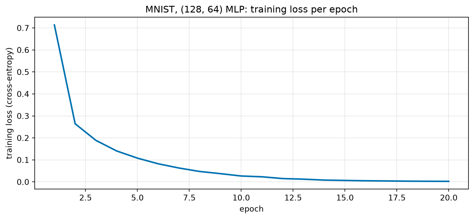
Read the warning. ConvergenceWarning means the epoch budget (max_iter=20) ran out while the training loss was still falling by more than tol per epoch. It is a statement about the optimizer, not about the model’s accuracy. Here the loss is still dropping, so the remedy is to raise max_iter – or to decide, from held-out data, that further training is not worth it.

Training Loss Curve

Code
fig, ax = plt.subplots(figsize=(10, 4))
ax.plot(np.arange(1, mlp.n_iter_ + 1), mlp.loss_curve_, color=OKABE_ITO[5], lw=2)
ax.set_xlabel('epoch')
ax.set_ylabel('training loss (cross-entropy)')
ax.set_title('MNIST, (128, 64) MLP: training loss per epoch')
ax.grid(alpha=0.3)
plt.show()

A fast drop, then a smooth flattening: the optimizer is fitting the training data, and has not quite finished (hence the warning). This curve says nothing about data the model has not seen – for that we need a held-out set.

Evaluate Performance

Code
from sklearn.metrics import accuracy_score, classification_report

y_pred = mlp.predict(X_test_scaled)
print(f"Training accuracy: {mlp.score(X_train_scaled, y_train):.4f}")
print(f"Test accuracy:     {accuracy_score(y_test, y_pred):.4f}")
Training accuracy: 1.0000
Test accuracy:     0.9555

Training accuracy 1.0, test accuracy about 0.96: the network fits its training set perfectly. A gap like this is the first hint of overfitting – we come back to it below.

Confusion Matrix

Code
from sklearn.metrics import confusion_matrix, ConfusionMatrixDisplay

fig, ax = plt.subplots(figsize=(8, 6))
cm = confusion_matrix(y_test, y_pred)
disp = ConfusionMatrixDisplay(confusion_matrix=cm, display_labels=mlp.classes_)
disp.plot(ax=ax, cmap='Blues', values_format='d')
plt.title('Confusion Matrix for MNIST Classification')
plt.show()
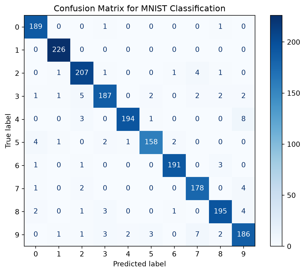
Rows are true digits, columns predictions. The largest off-diagonal cells are the shapes you would expect: true 4 read as 9 (8 times), true 9 read as 7 (7), and true 3 read as 2 (5).

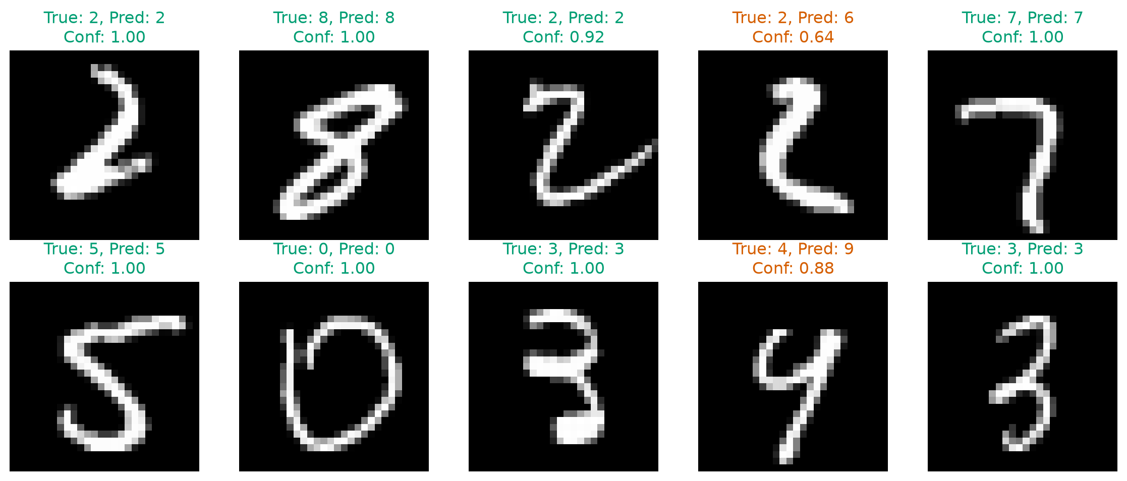
Visualize Predictions

Code
y_pred_proba = mlp.predict_proba(X_test_scaled)

fig, axes = plt.subplots(2, 5, figsize=(12, 5))
for i, ax in enumerate(axes.flat):
    ax.imshow(X_test[i].reshape(28, 28), cmap='gray')
    pred_label = y_pred[i]
    true_label = y_test[i]
    confidence = y_pred_proba[i].max()

    color = OKABE_ITO[2] if pred_label == true_label else OKABE_ITO[3]
    ax.set_title(f'True: {true_label}, Pred: {pred_label}\nConf: {confidence:.2f}',
                 color=color)
    ax.axis('off')
plt.tight_layout()
plt.show()
Regression Example

California Housing Dataset

Let’s predict house prices using MLP regression:

from sklearn.datasets import fetch_california_housing
from sklearn.preprocessing import StandardScaler
from sklearn.neural_network import MLPRegressor

# Load housing data
housing = fetch_california_housing()
X_housing = housing.data
y_housing = housing.target

print(f"Dataset shape: {X_housing.shape}")
print(f"Features: {housing.feature_names}")
Dataset shape: (20640, 8)
Features: ['MedInc', 'HouseAge', 'AveRooms', 'AveBedrms', 'Population', 'AveOccup', 'Latitude', 'Longitude']

Target: Median house value (in $100,000s)

Prepare Data and Define Model

# Split and scale
X_train_h, X_test_h, y_train_h, y_test_h = train_test_split(
    X_housing, y_housing, test_size=0.2, random_state=42
)

scaler = StandardScaler()
X_train_h_scaled = scaler.fit_transform(X_train_h)
X_test_h_scaled = scaler.transform(X_test_h)

# Train MLP Regressor with early stopping
mlp_reg = MLPRegressor(
    hidden_layer_sizes=(100, 50),
    activation='relu',
    solver='adam',
    alpha=0.001,
    batch_size=32,
    max_iter=100,
    early_stopping=True,
    validation_fraction=0.1,
    n_iter_no_change=10,
    random_state=42,
    verbose=False
)

Train the model

mlp_reg.fit(X_train_h_scaled, y_train_h)
print(f"Training stopped at epoch {mlp_reg.n_iter_} of max_iter={mlp_reg.max_iter}")
print(f"Best validation R²: {mlp_reg.best_validation_score_:.4f}")
Training stopped at epoch 76 of max_iter=100
Best validation R²: 0.7935

With early_stopping=True, scikit-learn holds out 10% of the training rows, scores them (\(R^2\)) after every epoch, stops once that score has not improved for 10 epochs, and keeps the best weights.

Training and Validation Curves

Code
epochs = np.arange(1, mlp_reg.n_iter_ + 1)
best_epoch_h = int(np.argmax(mlp_reg.validation_scores_)) + 1

fig, axes = plt.subplots(1, 2, figsize=(12, 4))
axes[0].plot(epochs, mlp_reg.loss_curve_, color=OKABE_ITO[5], lw=2)
axes[0].set_xlabel('epoch')
axes[0].set_ylabel('training loss (½ MSE + L2 penalty)')
axes[0].set_title('Housing MLP: training loss')
axes[0].grid(alpha=0.3)

axes[1].plot(epochs, mlp_reg.validation_scores_, color=OKABE_ITO[0], lw=2)
axes[1].axvline(best_epoch_h, color='gray', ls='--',
                label=f'best validation epoch ({best_epoch_h})')
axes[1].set_xlabel('epoch')
axes[1].set_ylabel('validation $R^2$ (10% held out)')
axes[1].set_title('Housing MLP: validation score')
axes[1].legend(loc='lower right')
axes[1].grid(alpha=0.3)
plt.tight_layout()
plt.show()
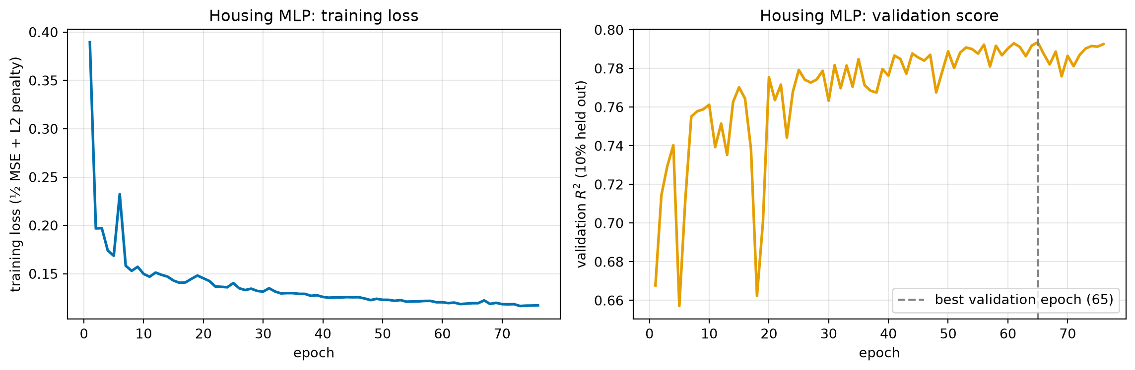
The training loss is noisy because each step uses a mini-batch of 32 rows (adam recovers from the bumps). The validation score is what early stopping watches: it peaked at the dashed line, and after 10 more epochs without improvement training stopped.

Evaluate Regression Model

from sklearn.metrics import mean_squared_error, r2_score, mean_absolute_error

# Make predictions
y_pred_h = mlp_reg.predict(X_test_h_scaled)

# Calculate metrics
mse = mean_squared_error(y_test_h, y_pred_h)
rmse = np.sqrt(mse)
mae = mean_absolute_error(y_test_h, y_pred_h)
r2 = r2_score(y_test_h, y_pred_h)

print(f"Root Mean Squared Error: {rmse:.4f}")
print(f"Mean Absolute Error: {mae:.4f}")
print(f"R² Score: {r2:.4f}")
Root Mean Squared Error: 0.5138
Mean Absolute Error: 0.3460
R² Score: 0.7986

An \(R^2\) of ~0.8 means our model explains 80% of the variance in house prices!

Predictions vs Actual

Code
fig, axes = plt.subplots(1, 2, figsize=(10, 5))

axes[0].scatter(y_test_h, y_pred_h, alpha=0.4, s=8, color=OKABE_ITO[5])
axes[0].plot([y_test_h.min(), y_test_h.max()],
             [y_test_h.min(), y_test_h.max()], color=OKABE_ITO[3], ls='--', lw=2)
axes[0].set_xlabel('Actual value ($100k)')
axes[0].set_ylabel('Predicted value ($100k)')
axes[0].set_title('Predicted vs Actual House Prices')
axes[0].grid(alpha=0.3)

residuals = y_test_h - y_pred_h
axes[1].scatter(y_pred_h, residuals, alpha=0.4, s=8, color=OKABE_ITO[5])
axes[1].axhline(y=0, color=OKABE_ITO[3], linestyle='--', lw=2)
axes[1].set_xlabel('Predicted value ($100k)')
axes[1].set_ylabel('Residual ($100k)')
axes[1].set_title('Residual Plot')
axes[1].grid(alpha=0.3)

plt.tight_layout()
plt.show()
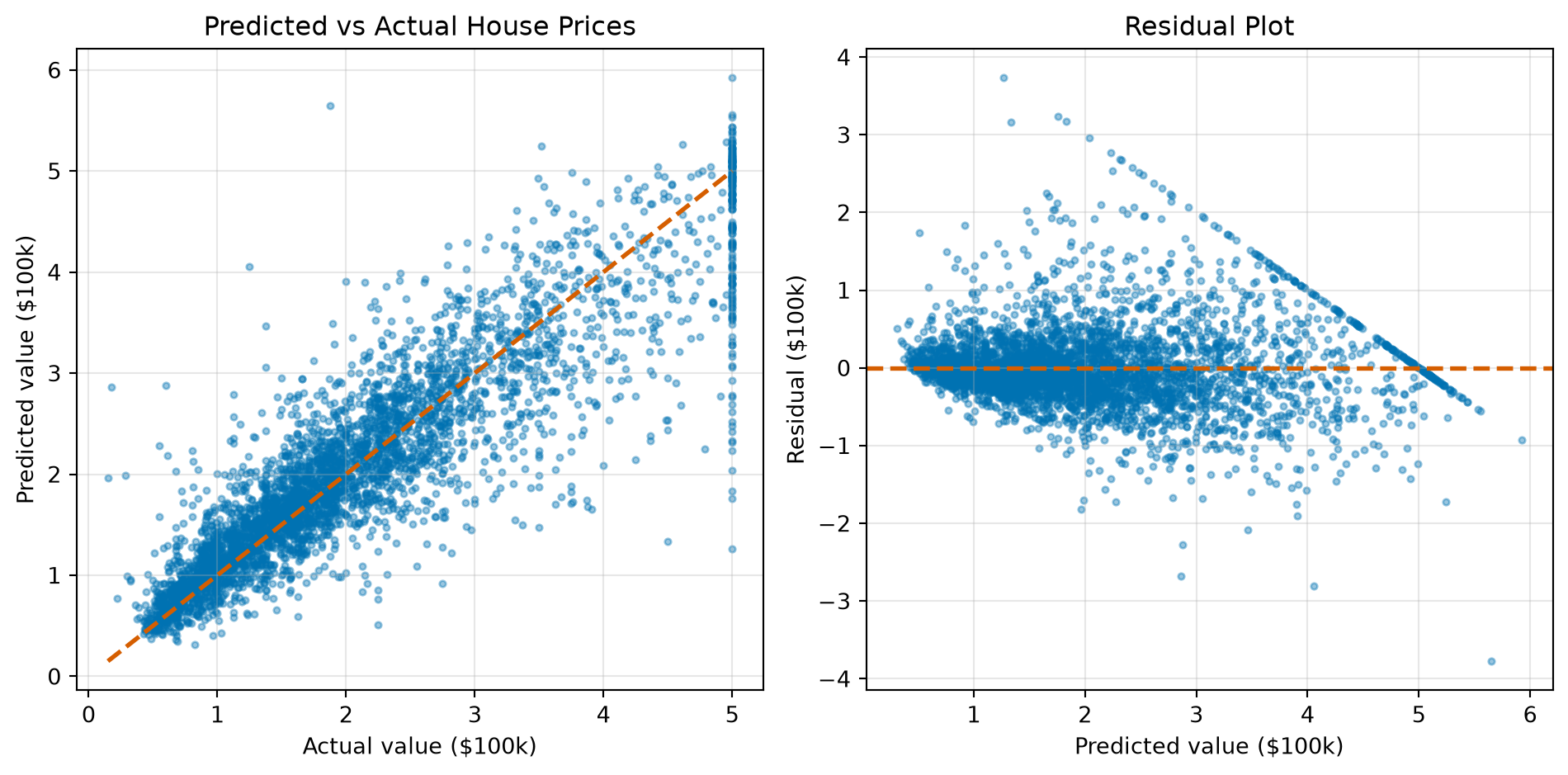
The vertical wall at 5 and the diagonal streak in the residuals are not the network’s doing: the source data caps the target at $500k, so every house worth more is recorded as 5.0 (about 5% of districts).

Why Scaling Matters

The same (64,) network on housing, fitted on standardized and on raw features:

fits = {}
for name, (A_tr, A_te) in {'standardized': (X_train_h_scaled, X_test_h_scaled),
                           'raw': (X_train_h, X_test_h)}.items():
    with warnings.catch_warnings():
        # both runs use a fixed 100-epoch budget; the standardized one uses all of it
        warnings.simplefilter('ignore', ConvergenceWarning)
        m = MLPRegressor(hidden_layer_sizes=(64,), max_iter=100, random_state=42)
        m.fit(A_tr, y_train_h)
    fits[name] = m
    print(f"{name:12s}: epochs {m.n_iter_:3d}   first-epoch loss {m.loss_curve_[0]:9.2f}"
          f"   test R² {m.score(A_te, y_test_h):.3f}")
standardized: epochs 100   first-epoch loss      3.06   test R² 0.762
raw         : epochs  80   first-epoch loss  29897.80   test R² 0.449

Why Scaling Matters, cont.

Code
fig, ax = plt.subplots(figsize=(10, 4))
for (name, m), c in zip(fits.items(), [OKABE_ITO[5], OKABE_ITO[3]]):
    ax.plot(np.arange(1, m.n_iter_ + 1), m.loss_curve_, color=c, lw=2, label=name)
ax.set_yscale('log')
ax.set_xlabel('epoch')
ax.set_ylabel('training loss (log scale)')
ax.set_title('Housing, (64,) MLP: standardized vs raw features')
ax.legend()
ax.grid(alpha=0.3, which='both')
plt.show()
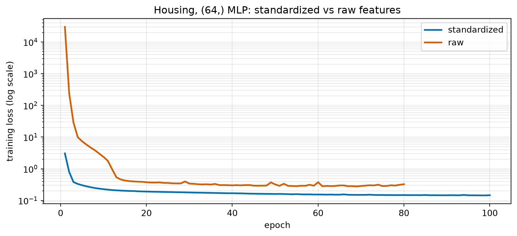
Raw Population runs into the tens of thousands while MedInc is near 4, so a few columns dominate every weighted sum and every gradient. The raw fit starts with an enormous loss, stalls, and stops “because it stopped improving” at a much worse \(R^2\).

Hyperparameter Tuning

Grid Search for Optimal Architecture

scikit-learn provides GridSearchCV for hyperparameter tuning:

Create a model without certain hyperparameters.

# Create MLP
mlp_grid = MLPClassifier(
    max_iter=20,
    random_state=42,
    early_stopping=True,
    validation_fraction=0.1,
    n_iter_no_change=5,
    verbose=False
)

# Use subset for faster demo
X_grid = X_train_scaled[:1500]
y_grid = y_train[:1500]

Grid Search, cont.

Define the parameter grid and run the grid search.

from sklearn.model_selection import GridSearchCV

# Define parameter grid
param_grid = {
    'hidden_layer_sizes': [(50,), (100,), (50, 50)],
    'activation': ['relu'],
    'alpha': [0.0001, 0.001]
}

grid_search = GridSearchCV(mlp_grid, param_grid, cv=3, n_jobs=2, verbose=0)
grid_search.fit(X_grid, y_grid)

print(f"Best parameters: {grid_search.best_params_}")
print(f"Best CV score: {grid_search.best_score_:.4f}")
Best parameters: {'activation': 'relu', 'alpha': 0.001, 'hidden_layer_sizes': (50,)}
Best CV score: 0.8740

Grid Search Results

Code
results_df = pd.DataFrame(grid_search.cv_results_)
ranked = (results_df
          .sort_values('rank_test_score')
          .assign(hidden_layer_sizes=lambda d: d['param_hidden_layer_sizes'].astype(str),
                  alpha=lambda d: d['param_alpha'])
          [['rank_test_score', 'hidden_layer_sizes', 'alpha',
            'mean_test_score', 'std_test_score']]
          .rename(columns={'rank_test_score': 'rank',
                           'mean_test_score': 'mean CV accuracy',
                           'std_test_score': 'std across folds'}))
best = ranked.iloc[0]
within = (ranked['mean CV accuracy'] >= best['mean CV accuracy'] - best['std across folds']).sum()
print(ranked.to_string(index=False, float_format='{:.4f}'.format))
print(f"\nConfigurations within one std of the best: {within} of {len(ranked)}")
 rank hidden_layer_sizes  alpha  mean CV accuracy  std across folds
    1              (50,) 0.0010            0.8740            0.0075
    2              (50,) 0.0001            0.8720            0.0082
    3             (100,) 0.0001            0.8707            0.0164
    4             (100,) 0.0010            0.8693            0.0159
    4           (50, 50) 0.0010            0.8693            0.0106
    6           (50, 50) 0.0001            0.8607            0.0164

Configurations within one std of the best: 5 of 6

Read the spread, not just the winner: five of the six configurations score within one standard deviation (0.0075) of the best, and even the last one’s own spread reaches it. On 1,500 samples the grid cannot tell them apart – pick the simplest.

Diagnosing Training

A Small, Fast Testbed

The experiments below use sklearn’s 8×8 digits (load_digits: 1,797 images, 64 pixel features with values 0–16) – a different, much smaller dataset than MNIST. Every fit takes under a second, and the in-class activity uses the same split.

from sklearn.datasets import load_digits
from sklearn.metrics import log_loss

SEED = 701
digits = load_digits()
Xd_train, Xd_test, yd_train, yd_test = train_test_split(
    digits.data, digits.target, test_size=0.3,
    stratify=digits.target, random_state=SEED)

scaler_d = StandardScaler().fit(Xd_train)
Xd_train_s = scaler_d.transform(Xd_train)
Xd_test_s = scaler_d.transform(Xd_test)
digit_classes = np.unique(digits.target)
print(f"train {Xd_train_s.shape}, test {Xd_test_s.shape}")
train (1257, 64), test (540, 64)

Reading the Learning Rate from the Loss Curve

Same (64,) network, same 60-epoch budget, three values of learning_rate_init:

Code
lr_settings = [(1e-5, 'too low'), (1e-3, 'just right'), (1.0, 'too high')]
fig, axes = plt.subplots(1, 3, figsize=(14.5, 4), sharey=True)
for ax, (lr, label), color in zip(axes, lr_settings, [OKABE_ITO[1], OKABE_ITO[2], OKABE_ITO[3]]):
    with warnings.catch_warnings():
        # the first two runs use the whole 60-epoch budget on purpose
        warnings.simplefilter('ignore', ConvergenceWarning)
        m = MLPClassifier(hidden_layer_sizes=(64,), learning_rate_init=lr,
                          max_iter=60, random_state=SEED).fit(Xd_train_s, yd_train)
    ax.plot(m.loss_curve_, color=color, lw=2.5)
    ax.set_title(f"{label} (lr = {lr:g})\ntest acc {m.score(Xd_test_s, yd_test):.3f}, "
                 f"{m.n_iter_} epochs")
    ax.set_xlabel('epoch')
    ax.grid(alpha=0.3)
    if label == 'too high':
        ax.text(8, 1.4, f"starts at {m.loss_curve_[0]:.0f}, bounces,\nstalls, stops early")
axes[0].set_ylabel('training loss (y-axis clipped)')
axes[0].set_ylim(0, 3.2)
plt.tight_layout()
plt.show()
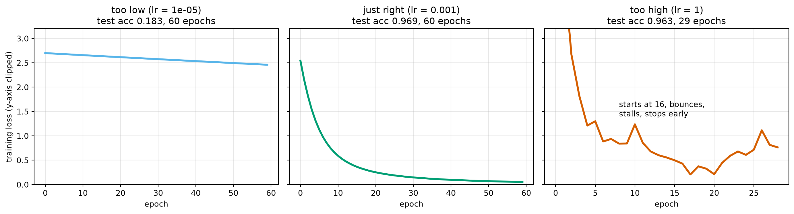
  • Too low: a nearly straight, slowly falling line – thousands of epochs from done.
  • Just right: fast drop, smooth flattening.
  • Too high: starts absurdly high, goes up on several epochs, stalls at a mediocre loss, and stops early because “it stopped improving”. It happened to score well – another seed may not.

Overfitting: What the Training Curve Cannot Show

A (512, 512) network with no L2 penalty, trained on 50 digits. To watch held-out loss epoch by epoch we train with partial_fit, which runs exactly one pass over the data per call:

idx_tiny, idx_val = train_test_split(np.arange(len(yd_train)), train_size=50,
                                     stratify=yd_train, random_state=SEED)
X_tiny, y_tiny = Xd_train_s[idx_tiny], yd_train[idx_tiny]
X_val, y_val = Xd_train_s[idx_val], yd_train[idx_val]

big = MLPClassifier(hidden_layer_sizes=(512, 512), alpha=0.0, random_state=SEED)
train_loss, val_loss = [], []
for epoch in range(200):
    big.partial_fit(X_tiny, y_tiny, classes=digit_classes)   # one epoch
    train_loss.append(log_loss(y_tiny, big.predict_proba(X_tiny), labels=digit_classes))
    val_loss.append(log_loss(y_val, big.predict_proba(X_val), labels=digit_classes))
best_epoch = int(np.argmin(val_loss))
print(f"train acc {big.score(X_tiny, y_tiny):.3f}   validation acc {big.score(X_val, y_val):.3f}")
train acc 1.000   validation acc 0.857

Overfitting, cont.

Code
fig, ax = plt.subplots(figsize=(10, 4.2))
ax.plot(train_loss, color=OKABE_ITO[5], lw=2.5,
        label='training loss (the 50 samples it trains on)')
ax.plot(val_loss, color=OKABE_ITO[0], lw=2.5,
        label=f'validation loss ({len(y_val)} digits it has never seen)')
ax.axvline(best_epoch, color='gray', ls='--',
           label=f'validation minimum (epoch {best_epoch})')
ax.annotate('training loss -> 0:\nthe samples are memorized', xy=(60, 0.0),
            xytext=(70, 0.9), arrowprops=dict(arrowstyle='->', color='gray'))
ax.annotate('validation loss stops improving\nand drifts back up', xy=(120, val_loss[120]),
            xytext=(95, 1.4), arrowprops=dict(arrowstyle='->', color='gray'))
ax.set_ylim(0, None)
ax.set_xlabel('epoch')
ax.set_ylabel('cross-entropy loss')
ax.set_title('(512, 512) network, 50 training digits, alpha = 0')
ax.legend(loc='upper right')
ax.grid(alpha=0.3)
plt.show()
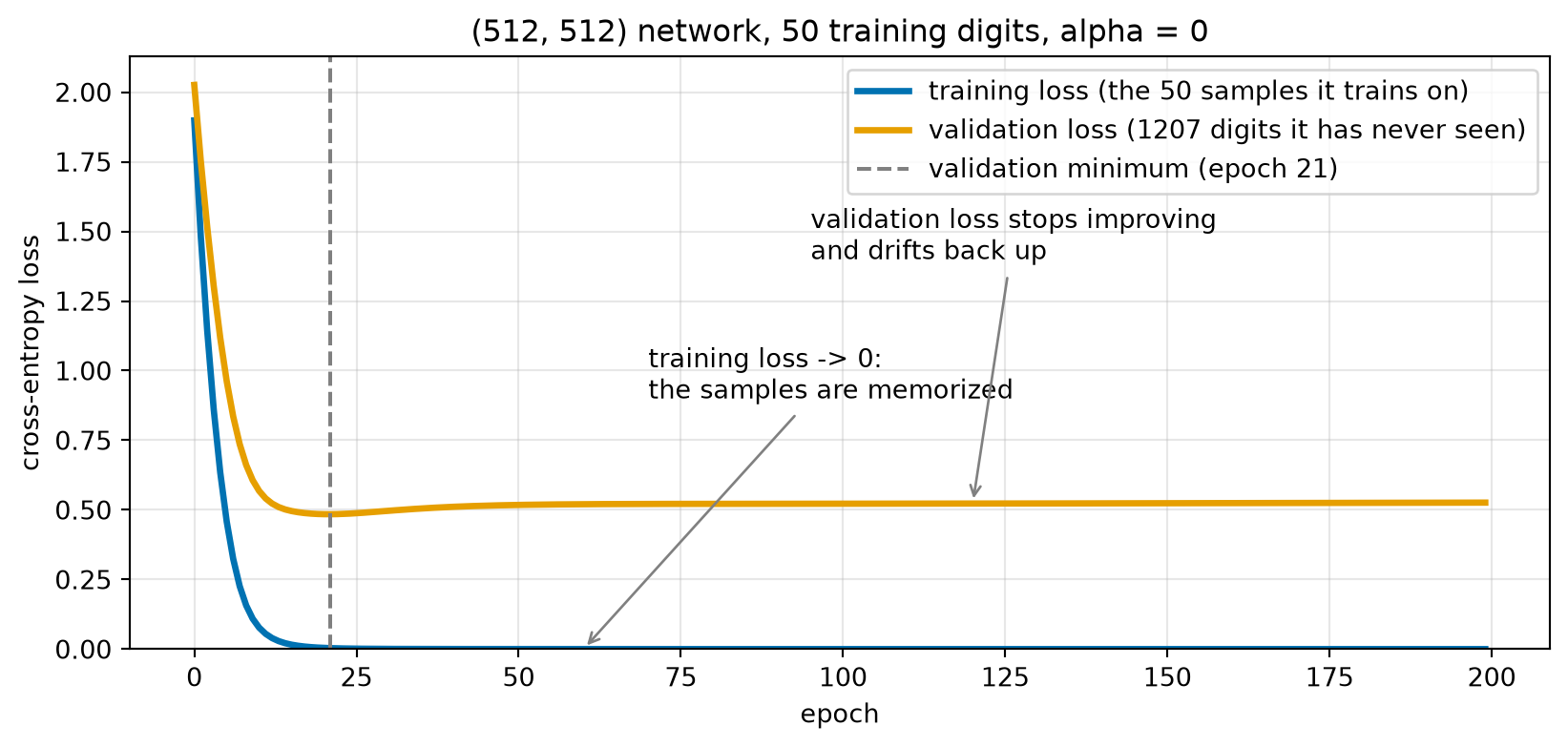
About 300K weights, 50 training samples: the network memorizes them (training loss → 0, training accuracy 1.0), while loss on unseen digits bottoms out early and creeps back up. loss_curve_ alone would have said “learning nicely”.

Overfitting: Diagnose, Then Repair

Diagnose by measuring on data the optimizer never saw: a validation split (as above), or cross-validation (cross_val_score, GridSearchCV) for a less noisy estimate. These measure overfitting; they do not change the model.

Repair – four levers, each changing something different:

repair scikit-learn what it changes
L2 regularization alpha=0.01 (default 1e-4) the objective: large weights cost more
early stopping early_stopping=True, validation_fraction=0.1, n_iter_no_change=10 the training loop: stop on validation evidence
smaller network e.g. hidden_layer_sizes=(64,) instead of (512, 512) the capacity: fewer weights to memorize with
more data more training rows the information: more constraints per weight

Regularizers trade variance for bias; only more data adds information. In the case study you will decide which of these levers to pull first for a client’s digit reader, and why.

Best Practices

Data Preprocessing

Always preprocess your data!

  1. Scale features: Use StandardScaler or normalize to [0, 1]
  2. Handle missing values: Impute or remove
  3. Encode categorical variables: One-hot encoding
  4. Use pipelines: Ensures consistent preprocessing
from sklearn.pipeline import Pipeline

pipeline = Pipeline([
    ('scaler', StandardScaler()),
    ('mlp', MLPClassifier(hidden_layer_sizes=(100,)))
])

pipeline.fit(X_train, y_train)

Architecture Selection

Rules of thumb for architecture:

  1. Start simple: Try single hidden layer first
  2. Layer sizes: Between input and output dimensions
  3. Depth vs width:
    • More layers → learn complex patterns
    • But risk overfitting on small data (as the (512, 512) net just did)
  4. Typical architectures:
    • Small data: (100,) or (50, 50)
    • Medium data: (100, 50) or (128, 64, 32)
    • Large data: Consider PyTorch

Solver Selection

Different solvers for different scenarios:

Solver Best For Notes
'adam' Most cases Good default, adaptive learning rate
'sgd' Large datasets Classic mini-batch SGD
'lbfgs' Small datasets Faster for small data, more memory
Code
solvers = ['adam', 'sgd', 'lbfgs']
results = {}

for solver in solvers:
    with warnings.catch_warnings():
        # all three hit the deliberately short 50-iteration budget
        warnings.simplefilter('ignore', ConvergenceWarning)
        m = MLPClassifier(hidden_layer_sizes=(50,), solver=solver,
                          max_iter=50, random_state=42)
        m.fit(X_train_scaled[:2000], y_train[:2000])
    results[solver] = m.score(X_test_scaled, y_test)
    print(f"{solver:6s}: test acc {results[solver]:.4f}   final training loss {m.loss_:.4f}")
adam  : test acc 0.9000   final training loss 0.0586
sgd   : test acc 0.8330   final training loss 0.6617
lbfgs : test acc 0.8800   final training loss 0.0010

sgd lost because its default learning_rate_init=0.001 is too small for a 50-epoch budget – its training loss is still high, the “too low” picture above. For lbfgs, max_iter counts full-batch quasi-Newton iterations, not epochs, so this is not a like-for-like budget (and lbfgs records no loss_curve_).

Common Issues

ConvergenceWarning: match the remedy to the curve

  • Curve still falling at the end → raise max_iter (the budget ran out).
  • Curve bouncing up and down → lower learning_rate_init (steps too big). If it is merely slow, a smaller rate makes it worse.
  • Curve flat but the warning persists → stop on evidence with early_stopping=True / n_iter_no_change. This changes the stopping rule; it does not make the optimizer converge.
  • Loss huge from epoch 1 → check scaling.

Poor Performance

If accuracy is low:

  1. Is data scaled/normalized?
  2. Is architecture appropriate?
  3. Is learning rate too high/low?
  4. Do you need more iterations?
  5. Is regularization too strong?

What scikit-learn’s MLP Cannot Do

scikit-learn’s MLP is a fully connected network with a fixed recipe. It initializes weights with Glorot (Xavier) scaling – the fix from the Neural Networks I activity – and offers L2 and early stopping, but nothing else:

  • no dropout or batch normalization
  • no learning-rate warm-up or custom schedules (beyond sgd’s three)
  • no GPU, no custom losses or layers
  • no convolutional or recurrent layers for images and sequences

For those you move to PyTorch: see Module M4: CNNs and Module M3: RNNs, and DS542, Deep Learning for Data Science.

Summary

Summary

You can now:

  1. Map the ideas from Neural Networks I onto scikit-learn’s knobs – hidden_layer_sizes, learning_rate_init, batch_size, max_iter, alpha, solver – and say what turning each one up does.
  2. Run the training recipe properly: scale inputs (fit the scaler on the training split), fit MLPClassifier/MLPRegressor, evaluate on held-out data – and explain why unscaled features break gradient training.
  3. Read a loss curve: it shows training loss only; recognize too-low, healthy and too-high learning rates by shape, and match each ConvergenceWarning remedy to the curve.
  4. Diagnose overfitting from training vs validation loss, and repair it with alpha, early stopping, a smaller network or more data.
  5. Choose between scikit-learn and PyTorch for a given problem, and name what would flip the choice.

To Dig Deeper

Other modules in the course notes:

Additional resources: