Recap: Decision Trees and Random Forests
DS701 Session 9 — Mon Oct 5, 2026
2. Where can a split go? Depends on the attribute type
- Binary — one obvious split.
- Nominal — multi-way (a branch per value) or binary (a partition of the values into two groups); \(\mathcal{O}(2^k)\) groupings to search.
- Ordinal — binary splits are fine if the ordering is preserved:
{Small, Medium} | {Large, X-Large}is legal,{Small, Large} | {Medium, X-Large}is not. - Continuous — threshold \(x \le \tau\): sort, then sweep the midpoints between consecutive values, \(\mathcal{O}(n)\) after the sort.
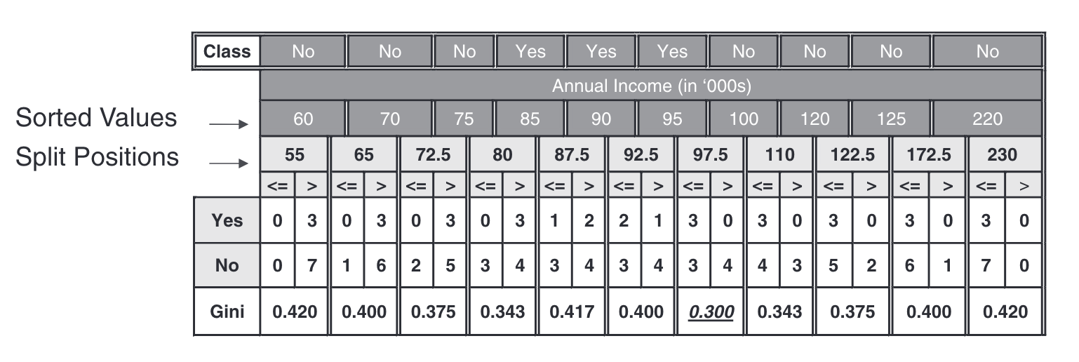
Pick the threshold with the lowest weighted impurity.
3. Impurity measures and how a split is scored
\[ \begin{aligned} \textnormal{Gini} &= 1 - \sum_{i=0}^{c-1} p_i(t)^2 \\ \textnormal{Entropy} &= -\sum_{i=0}^{c-1} p_i(t) \log_2 p_i(t) \\ \textnormal{Error} &= 1 - \max_i p_i(t) \end{aligned} \]
\(p_i(t)\) = relative frequency of class \(i\) at node \(t\); \(0 \log_2 0 = 0\).
Score a split by the weighted average over its children and take the largest gain:
\[ I(\textnormal{ch}) = \sum_{j=1}^{k} \frac{N(v_j)}{N} I(v_j), \quad \Delta = I(\textnormal{parent}) - I(\textnormal{ch}) \]
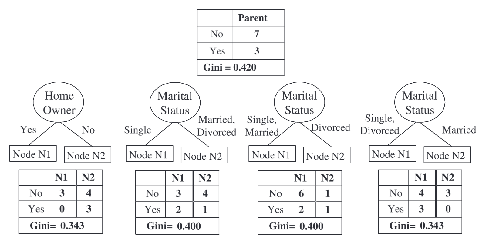
- All three are 0 for a pure node, maximal for a uniform mix.
- Entropy \(\ge\) Gini \(\ge\) Error, always.
- Gini and entropy almost always pick the same split; Gini is cheaper (no logs) and is
scikit-learn’s default. - Largest gain = smallest weighted child impurity, since the parent term is fixed.
5. Overfitting: bias, variance, and how to stop it
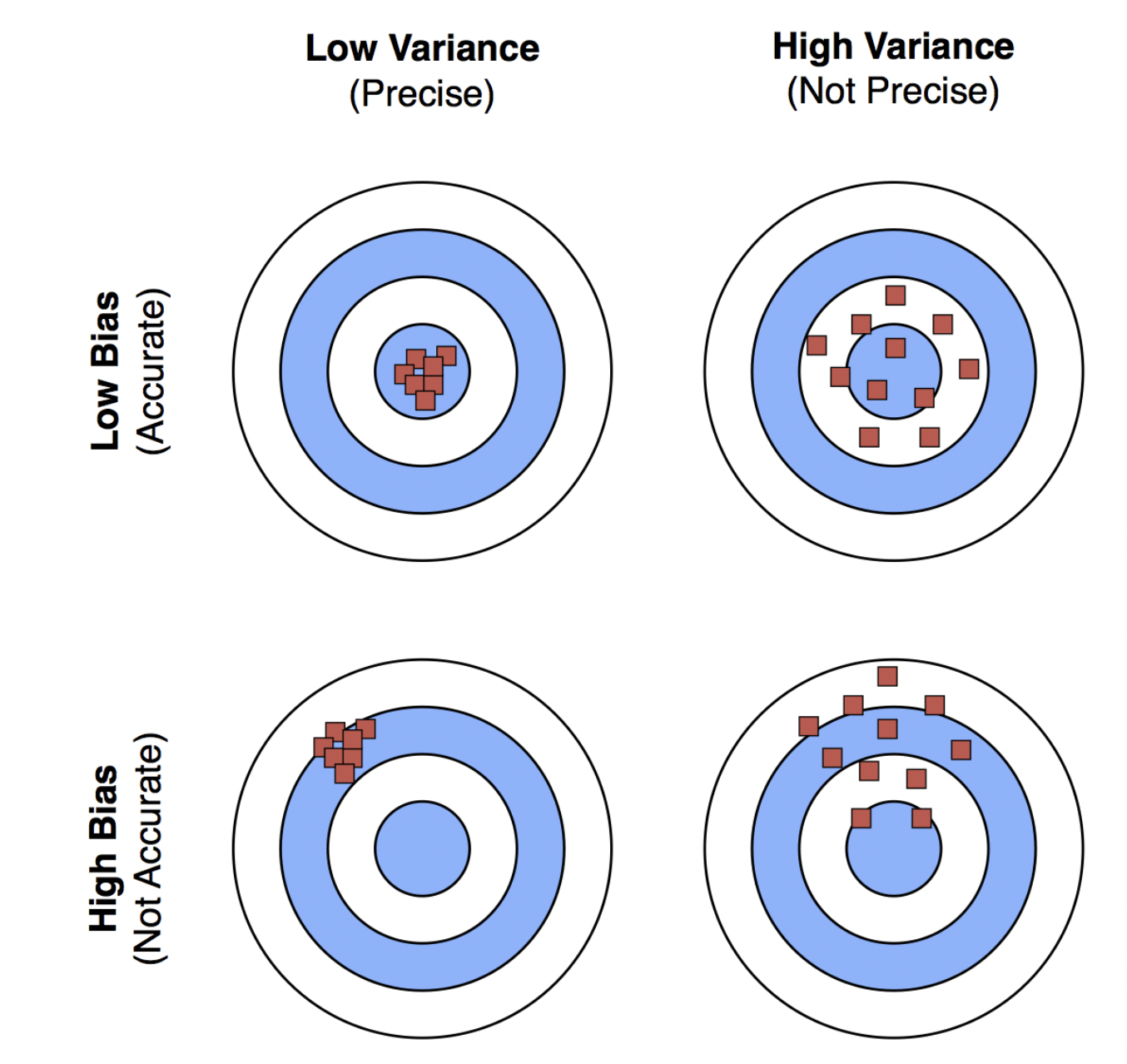
- Bias — error from an over-simple model; a depth-1 stump underfits.
- Variance — error from an over-complex model; a fully grown tree fits the training set exactly and its structure changes wildly under resampling.
- A fully grown tree is the canonical low-bias / high-variance learner — exactly the raw material ensembles want.
- Pre-prune (stopping criteria):
max_depth,min_samples_split/min_samples_leaf, minimum impurity decrease. - Post-prune: grow fully, then collapse subtrees that don’t pay for themselves on held-out data (
ccp_alpha). - On Titanic, both
min_samples_split=20andmax_depth=3beat the unrestricted tree on validation error — less tree, better model.
Case study: prioritizing breast biopsies with trees and forests
Goal: advise a consortium of Boston hospitals on whether nucleus measurements from breast biopsies can flag likely-malignant samples — find the best single cutoff, choose a tree depth that generalizes, and decide whether a random forest is worth giving up a readable tree.
- Work in groups of 2–3. Open the notebook for your section — the data split differs, so the other section’s numbers are wrong for you.
- Parts 1–3 are autograded and submitted to Gradescope.
- Finish with the report out: what you would tell the clinical team, and one takeaway to pair-share with a neighboring team.
- Staff will circulate — be ready to explain any part of your work.


The activity notebook goes live on the day of the lecture. Colab is optional — you can also open it on GitHub and run it locally.