You are a loan officer at Terrier Savings and Loan.
You have a dataset on loans that you have made in the past.
You want to build a model to predict whether a loan will default.
Loans Data Set
Code
import pandas as pdimport osimport urllib.requestdef data_file(path):"""Course data file: use a local copy (here, or in the repo root above a notebook in jupyter_notebooks/), else fetch it from the Materials repo (Colab)."""for prefix in ('', '../'):if os.path.exists(prefix + path):return prefix + path os.makedirs(os.path.dirname(path) or'.', exist_ok=True) urllib.request.urlretrieve('https://raw.githubusercontent.com/tools4ds/DS701-Materials-FA26/main/'+ path, path)return pathloans = pd.read_csv(data_file('data/loans.csv'), index_col=0)loans
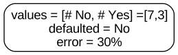
Looking at the table, let’s just start with the simplest model possible and just predict that no one will default.
So the output of our model is just to always predict “No”.
We see a 30% error rate since 3 out of 10 loans defaulted.
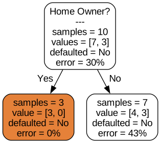
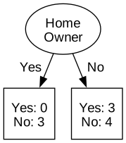
Let’s split the data based on the “Home Owner” field. (values = [# No, # Yes]).
We see that the left node (Home Owner == Yes) has a 0% error rate since all the samples are Defaulted == No. We don’t split this node since all the samples are of the same class. We call this node a leaf node and we’ll color it orange.
The right node (Home Owner == No) has a 43% error rate since 3 out of 7 loans defaulted.
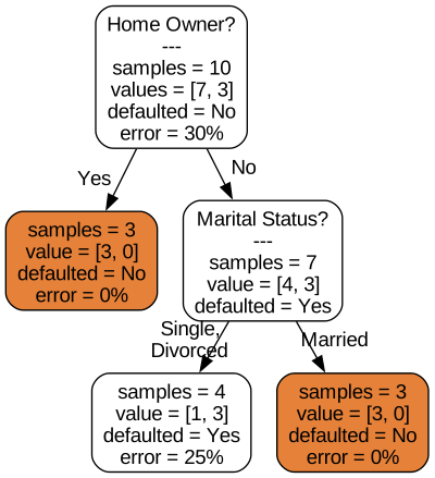
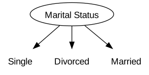
Let’s split this node into two nodes based on the Marital Status field.
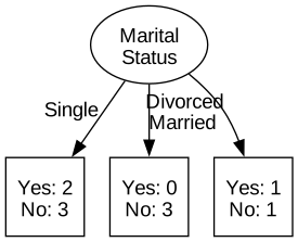
Let’s split on the “Marital Status” field.
We see that the 3 defaulted loans are all for single or divorced people. Since the node is all one class, we don’t split this node and we call it a leaf node.
We can list the subsets for the two criteria to calculate the error rate.
Table: Home Owner == No and Marital Status == Married –> Defaulted == No
Error rate for predicting Defaulted == No is 0%.
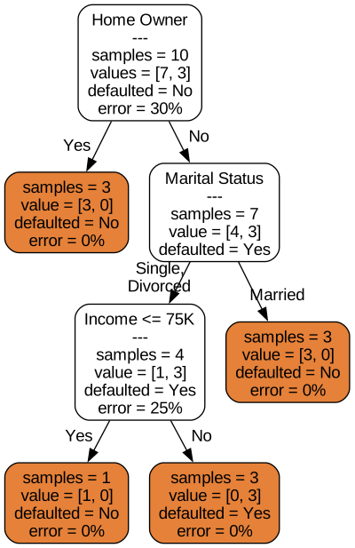
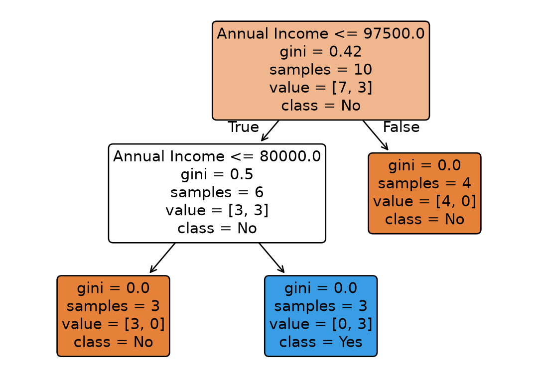
Let’s try to split on the “Annual Income” field.
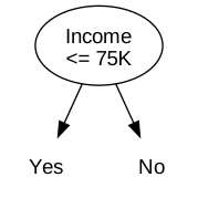
We see that the person with income of 70K doesn’t default, so we split the node into two nodes based on the “Income” field.
We arbitrarily pick a threshold of $75K.
Evaluating the Model
Evaluating the Model
We’ve dispositioned every data point by walking down the tree to a leaf node.
How do we know if this tree is good?
We arbitrarily picked the order of the fields to split on.
Is there a way to systematically pick the order of the fields to split on?
This is called the splitting criterion.
There’s also the question of when to stop splitting, or the stopping criterion.
So far, we stopped splitting when we reached a node of pure class but there are reasons to stop splitting even without pure classes, which we’ll see later.
Specifying the Test Condition
Before we continue, we should take a moment to consider how we specify a test condition of a node.
How we specify a test condition depends on the attribute type which can be:
Binary (Boolean)
Nominal (Categorical, e.g., cat, dog, bird)
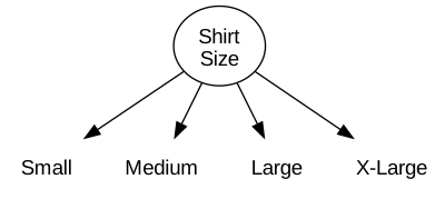
Ordinal (e.g., Small, Medium, Large)
Continuous (e.g., 1.5, 2.1, 3.7)
And depends on the number of ways to split:
multi-way
binary
For a Nominal (Categorical) attribute:
In a Multi-way split we can use as many partitions as there are distinct values of the attribute:
For a Nominal (Categorical) attribute:
In a Binary split we divide the values into two groups.
In this case, we need to find an optimal partitioning of values into groups, which we discuss shortly.
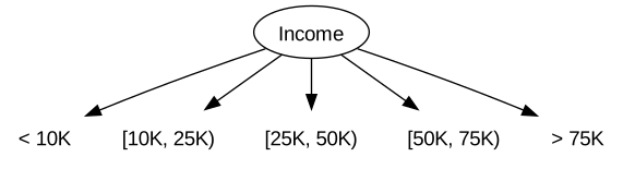
For an Ordinal attribute, we can use a multi-way split with as many partitions as there are distinct values.
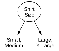
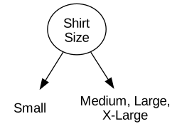
Or we can use a binary split as long we preserve the ordering of the values.
Warning
Be careful not to violate the ordering of values such as {Small, Large} and {Medium, X-Large}.
A Continuous attribute can be handled two ways:
It can be thresholded to form a binary split.
Or it can be split into contiguous ranges to form an ordinal categorical attribute.
Note that finding good partitions for \(k\) nominal attributes can be expensive, \(\mathcal{O}(2^k)\), possibly involving combinatorial searching of groupings.
However for ordinal or continuous attributes, sweeping through a range of \(n\) threshold values can be more efficient if \(n \approx k\). \(\mathcal{O}(n)\) for a sorted list.
Selecting Attribute and Test Condition
Ideally, we want to pick attributes and test conditions that maximize the homogeneity of the splits.
We can use an impurity index to measure the homogeneity in a node.
We’ll look at ways of measuring impurity of a node and then collective impurity of its child nodes.
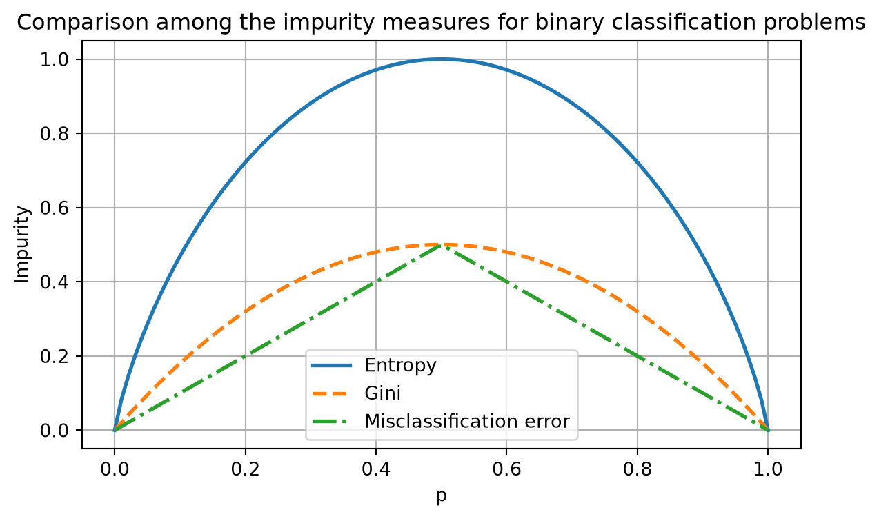
Node Impurity Measures
The following are three impurity indices, for a given node \(t\):
Let’s compute collective impurity on our loans dataset to see which feature to split on.
(a) Collective Entropy: 0.690
(b) Collective Entropy: 0.686
(c) Collective Entropy index: 0.00
Tip
Try calculating the collective Entropy for (a) and (b) and see if you get the same values.
Important
The collective entropy for (c) is 0. Why would we not want to use this node?
There are two ways to overcome this problem.
One way is to generate only binary decision trees, thus avoiding the difficulty of handling attributes with varying number of partitions. This strategy is employed by decision tree classifiers such as CART.
Another way is to modify the splitting criterion to take into account the number of partitions produced by the attribute. For example, in the C4.5 decision tree algorithm, a measure known as gain ratio is used to compensate for attributes that produce a large number of child nodes.
Having a low impurity value alone is insufficient to find a good attribute test condition for a node.
Having more child nodes can make a decision tree more complex and consequently more susceptible to overfitting.
Hence, the number of children produced by the splitting attribute should also be taken into consideration while deciding the best attribute test condition.
where \(N(v_i)\) is the number of samples assigned to node \(v_i\) and \(k\) is the number of child nodes.
The numerator is the gain \(\Delta\) with \(I = \text{Entropy}\), called the Information Gain: the reduction in entropy achieved by the split.
The denominator, Split Information, is the entropy of the child sizes, not of the classes. It grows when the split produces many equally-sized child nodes, and it does not depend on which impurity measure is used.
Gain Ratio: Changing Only the Numerator
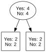
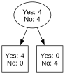
Parent node: 4 Yes, 4 No, so \(\text{Entropy(Parent)} = 1\). Both splits below make two children of 4 samples.
Same child sizes \(\Rightarrow\) same Split Info. Only the class labels inside the children changed, and the numerator rewards the purer split.
Gain Ratio: Changing Only the Denominator
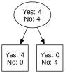
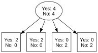
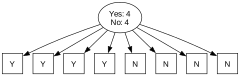
Same parent (4 Yes, 4 No). Now every split has pure children, but a different number of them.
(B) 2 children of 4
(C) 4 children of 2
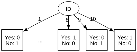
(D) 8 children of 1 (like ID)
(B) \(k=2\)
(C) \(k=4\)
(D) \(k=8\)
Info Gain (numerator)
\(1\)
\(1\)
\(1\)
Split Info (denominator)
\(-2\cdot\tfrac{1}{2}\log_2\tfrac{1}{2} = 1\)
\(-4\cdot\tfrac{1}{4}\log_2\tfrac{1}{4} = 2\)
\(-8\cdot\tfrac{1}{8}\log_2\tfrac{1}{8} = 3\)
Gain Ratio
\(\mathbf{1}\)
\(\mathbf{0.5}\)
\(\mathbf{0.33}\)
Information Gain cannot tell these apart. Split Info grows as \(\log_2 k\) for \(k\) equal-sized children, so the gain ratio penalizes the many-way split.
Split Info Depends Only on Child Sizes
Split Info is just the entropy of the child sizes; the class labels never enter it. For \(N = 8\) samples:
For a fixed number of children, Split Info is largest when they are equal-sized.
Caveat: a lopsided split (7, 1) has a small denominator, which can inflate the gain ratio. C4.5 only considers attributes whose information gain is at least average.
Gain Ratio Example
Let’s compare the Gain Ratio for Home Owner and Marital Status attributes using the loans dataset.
Recall from the earlier example that the parent node has 3 Yes and 7 No defaulters (10 total samples).
Although Marital Status has a slightly higher Information Gain, it has a lower Gain Ratio because it splits the data into 3 child nodes rather than 2.
The Gain Ratio penalizes attributes that create more splits, making Home Owner the preferred choice.
Option 1: Binary Splits Only (CART)
Gain ratio was C4.5’s fix for many-way splits (option 2). CART takes option 1 instead: every test condition is a binary split.
With every split binary, the many-children penalty is gone, so CART uses the plain gain \(\Delta\) rather than gain ratio.
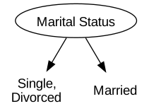
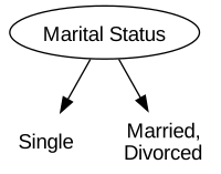
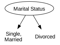
Binary splits also mean an attribute can have several candidate test conditions. A nominal attribute with \(k\) values has \(2^{k-1} - 1\) ways to group its values into two children, so Marital Status (3 values) has 3.
Choosing a split now means choosing the attribute and its test condition: we score every (attribute, grouping) pair and keep the best.
CART scores splits with Gini impurity. Entropy would also work and usually picks the same split. Gini is also scikit-learn’s default (criterion='gini'), which we’ll use below.
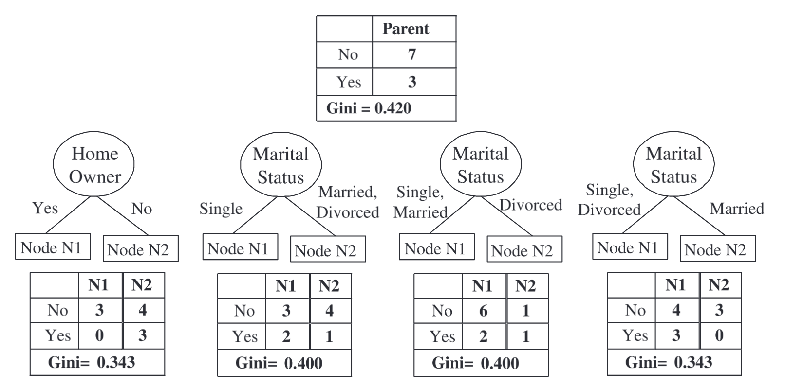
Ex: Best Binary Split Using Gini
The loans parent node (3 Yes, 7 No) has four candidate binary splits: one for Home Owner and three groupings of Marital Status.
We pick the split with the largest gain \(\Delta\), now with \(I = \text{Gini}\), i.e., the lowest collective Gini impurity.
Home Owner and Single+Divorced vs Marriedtie at 0.343: both produce children with 0/3 and 3/4 Yes/No counts.
Different test conditions can produce the same partition counts. A tree builder breaks such ties arbitrarily (scikit-learn by random feature order, set by random_state).
Ex: Computing the Gini Gains
Code
def gini_impurity(yes_count, no_count):"""Calculate Gini impurity for a node""" total = yes_count + no_countif total ==0:return0 p_yes = yes_count / total p_no = no_count / total gini =1- (p_yes**2+ p_no**2)return ginidef weighted_gini(n1_yes, n1_no, n2_yes, n2_no):"""Calculate weighted average Gini impurity after split""" n1_total = n1_yes + n1_no n2_total = n2_yes + n2_no total = n1_total + n2_total gini_n1 = gini_impurity(n1_yes, n1_no) gini_n2 = gini_impurity(n2_yes, n2_no) weighted_gini = (n1_total/total) * gini_n1 + (n2_total/total) * gini_n2return weighted_gini# Parent nodeparent_yes =3parent_no =7parent_gini = gini_impurity(parent_yes, parent_no)print("="*60)print("PARENT NODE")print("="*60)print(f"Yes: {parent_yes}, No: {parent_no}")print(f"Gini Impurity: {parent_gini:.3f}")print()# Define all four splitssplits = {"Home Owner": {"N1": {"yes": 0, "no": 3}, # Yes (owns home)"N2": {"yes": 3, "no": 4} # No (doesn't own home) },"Marital Status (Split 1: Single vs Married+Divorced)": {"N1": {"yes": 2, "no": 3}, # Single"N2": {"yes": 1, "no": 4} # Married, Divorced },"Marital Status (Split 2: Single+Married vs Divorced)": {"N1": {"yes": 2, "no": 6}, # Single, Married"N2": {"yes": 1, "no": 1} # Divorced },"Marital Status (Split 3: Single+Divorced vs Married)": {"N1": {"yes": 3, "no": 4}, # Single, Divorced"N2": {"yes": 0, "no": 3} # Married }}# Calculate for each splitresults = []for split_name, nodes in splits.items(): n1_yes = nodes["N1"]["yes"] n1_no = nodes["N1"]["no"] n2_yes = nodes["N2"]["yes"] n2_no = nodes["N2"]["no"] gini_n1 = gini_impurity(n1_yes, n1_no) gini_n2 = gini_impurity(n2_yes, n2_no) weighted_gini_value = weighted_gini(n1_yes, n1_no, n2_yes, n2_no) gini_gain = parent_gini - weighted_gini_value results.append({'name': split_name,'weighted_gini': weighted_gini_value,'gini_gain': gini_gain,'gini_n1': gini_n1,'gini_n2': gini_n2,'n1_yes': n1_yes,'n1_no': n1_no,'n2_yes': n2_yes,'n2_no': n2_no })print("="*60)print(f"SPLIT: {split_name}")print("="*60)print(f"Node N1: Yes={n1_yes}, No={n1_no}, Total={n1_yes+n1_no}")print(f" Gini(N1) = {gini_n1:.3f}")print(f"Node N2: Yes={n2_yes}, No={n2_no}, Total={n2_yes+n2_no}")print(f" Gini(N2) = {gini_n2:.3f}")print(f"\nWeighted Gini (after split): {weighted_gini_value:.3f}")print(f"Gini Gain: {gini_gain:.3f}")print()# Summary: Find best splitprint("="*60)print("SUMMARY - BEST SPLIT")print("="*60)results_sorted =sorted(results, key=lambda x: x['gini_gain'], reverse=True)for i, result inenumerate(results_sorted, 1):print(f"{i}. {result['name']}")print(f" Weighted Gini: {result['weighted_gini']:.3f}, Gini Gain: {result['gini_gain']:.3f}")print()best_gain = results_sorted[0]['gini_gain']best = [r['name'] for r in results_sorted if np.isclose(r['gini_gain'], best_gain)]print(f"Maximum Gini Gain: {best_gain:.3f}, achieved by:")for name in best:print(f" {name}")
Motivated around the idea that combining several noisy classifiers can result in a better prediction under certain conditions.
The base classifiers are independent
The base classifiers are noisy (high variance)
The base classifiers are low (ideally zero) bias
Bias and Variance
Recall bias and variance from Generalization: bias is error from a model too simple to capture the pattern (a shallow tree underfits); variance is error from a model so flexible that it changes with every training sample (a deep tree overfits).
A fully grown tree is low bias, high variance. Averaging many such trees keeps the low bias and averages away much of the variance – ensembles reduce variance.
Random Forests
Random forests are an ensemble of decision trees that:
Train each tree on a bootstrap sample: \(N\) points drawn with replacement from the \(N\) training points.
At each split, consider only a random subset of the features (max_features in scikit-learn).
Grow each tree to completion (low bias, high variance).
Take a majority vote of the trees to form the final prediction.
Note
Why not one tree on all the data? A deep tree’s problem is variance, not too little data. Averaging \(B\) trees with pairwise correlation \(\rho\) shrinks variance to \(\rho\sigma^2 + \frac{1-\rho}{B}\sigma^2\). The bootstrap and the feature subsampling exist to make the trees differ, which lowers \(\rho\).
Titanic Example
We’ll use the Titanic data set and excerpts of this Kaggle tutorial to illustrate the concepts of overfitting and random forests.
Code
import pandas as pddf_train = pd.read_csv(data_file('data/titanic/train.csv'), index_col='PassengerId')df_test = pd.read_csv(data_file('data/titanic/test.csv'), index_col='PassengerId')
There are 418 entries in the test set with same fields except for ‘Survived’, which is what we need to predict.
We’ll do some data cleaning and preparation.
Code
import numpy as npdef proc_data(df): df['Fare'] = df.Fare.fillna(0) df.fillna(modes, inplace=True) # Fill missing values with the mode df['LogFare'] = np.log1p(df['Fare']) # Create a new column for the log of the fare + 1 df['Embarked'] = pd.Categorical(df.Embarked) # Convert to categorical df['Sex'] = pd.Categorical(df.Sex) # Convert to categoricalmodes = df_train.mode().iloc[0] # Get the mode for each columnproc_data(df_train)proc_data(df_test)
Let’s split the independent (input) variables from the dependent (output) variable.
def xs_y(df): xs = df[cats+conts].copy()return xs,df[dep] if dep in df elseNonetrn_xs,trn_y = xs_y(trn_df)val_xs,val_y = xs_y(val_df)
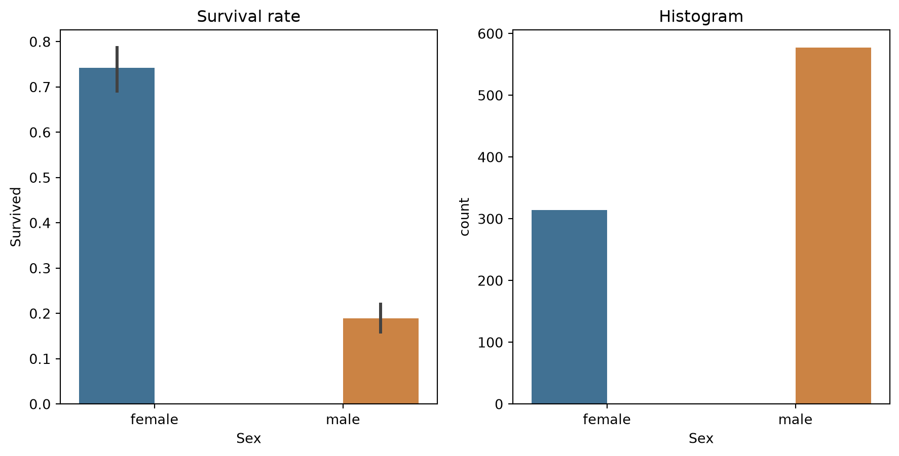
Here’s the predictions for our extremely simple model, where female is coded as 0:
preds = val_xs.Sex==0
We’ll use mean absolute error to measure how good this model is:
from sklearn.metrics import mean_absolute_errormean_absolute_error(val_y, preds)
0.21524663677130046
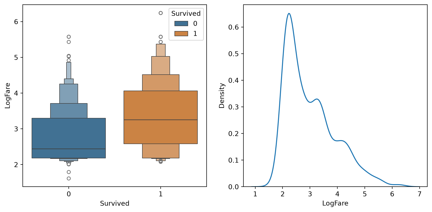
Alternatively, we could try splitting on a continuous column. We have to use a somewhat different chart to see how this might work – here’s an example of how we could look at LogFare:
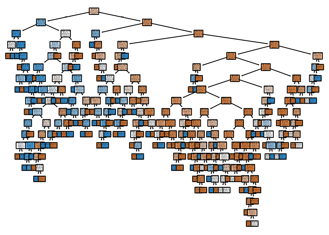
Better than the fully grown tree (0.265), but not better than our limited single trees (about 0.19). Why not?
Why Didn’t the Forest Win?
Its trees are grown to completion. With only 668 training passengers and 7 features, each deep tree memorizes noisy labels. A noisy passenger lands in about 63% of the bootstrap samples, so many trees memorize the same noise, and averaging cannot cancel what the trees share.
One validation set is a noisy judge. With 223 validation passengers and an error near 0.2, the standard error is \(\sqrt{0.2 \cdot 0.8 / 223} \approx 0.027\). A gap of 0.02 between two models is within that noise.
So: tune the forest, and choose its hyperparameters with cross-validation on the training data, not by checking the validation score (Generalization).
Tuning the Forest
Limit how small a leaf can be (min_samples_leaf), scoring each setting by repeated 5-fold cross-validation on the training data only.
The tuned forest has the lowest validation error in this lecture (0.175 vs. 0.188 for the best single tree), but by our own yardstick that gap is within the noise.
“Grow each tree to completion” is the default, not a rule. On small, noisy data a minimum leaf size helps, because averaging removes only the variance the trees don’t share.
Why so close? Titanic is small, has few features, and is dominated by one (Sex), so there is little variance left for averaging to remove. Forests pull further ahead with more data and more features.
Summary
Decision trees – five things we did:
Grow a tree greedily. At each node, try every (attribute, test condition) pair and keep the one with the largest gain \(\Delta = I(\textnormal{parent}) - I(\textnormal{children})\). The impurity \(I\) can be Gini, entropy, or classification error.
Handle many-way splits. Gain alone favors splits into many small children (the ID attribute). C4.5 divides by Split Info (gain ratio); CART allows only binary splits and uses the plain gain with Gini.
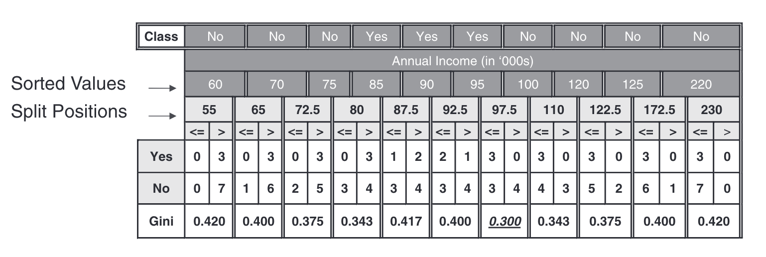
Split continuous attributes at a threshold \(\tau\), chosen by the same gain criterion.
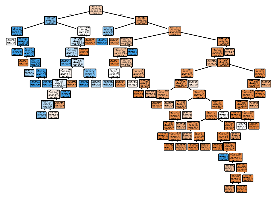
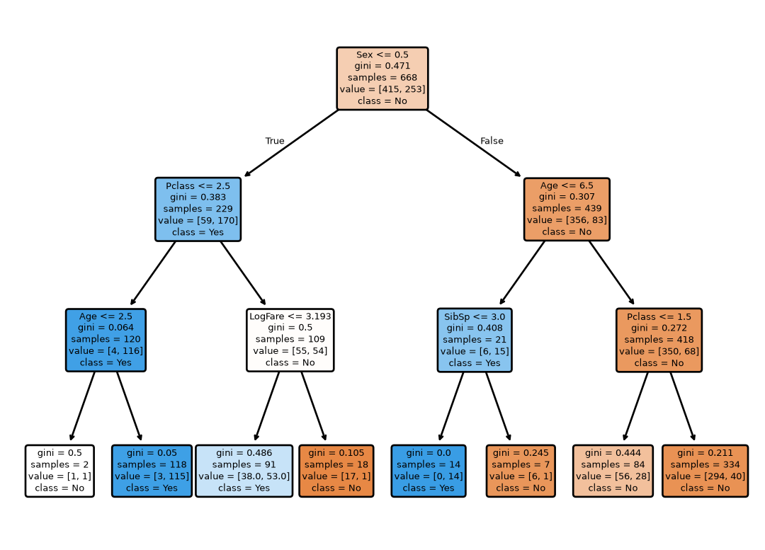
Control overfitting. On Titanic, the fully grown tree had a validation error of 0.265, worse than the one-rule “women survive” model (0.215). Stopping criteria (min_samples_split, max_depth) brought it down to about 0.19.
Reduce variance with random forests. Average many deep trees, each trained on a bootstrap sample with random feature subsets at every split. Untuned (0.211) it beat only the full tree; with min_samples_leaf chosen by cross-validation it reached 0.175, the lowest validation error in the lecture, though only narrowly.
Next: \(k\)-Nearest Neighbors Classifiers
Another classifier with the same bias–variance trade-off and a different knob: the number of neighbors \(k\) plays the role that depth played today.
Small \(k\) overfits, like a fully grown tree; large \(k\) underfits, like a stump.
We will also see why distance-based methods break down in high dimensions (the curse of dimensionality), and meet Naive Bayes.