Generalization: Why Training Error Lies

Introduction

Every supervised method in this course – trees, \(k\)-NN, regression, neural networks – is judged by one question: how well does it predict on data it has never seen?

Today we make that question precise, and see why the most natural answer (pick the model with the lowest training error) is wrong.

The Supervised Learning Problem

You are given some example data, which we’ll think of abstractly as tuples \(\{(\mathbf{x}_i, y_i)\,|\,i = 1,\dots,N\}\).
- \(\mathbf{x}_i\) are the inputs or independent variables. Its components are called features.
- \(y_i\) are the outputs or dependent variables (a.k.a. labels, targets or ground truth).
Your goal is to learn a rule that allows you to predict \(y_j\) for some \(\mathbf{x}_j\) that is not in the example data you were given.
The collection \(\{(\mathbf{x}_i, y_i)\,|\,i = 1,\dots,N\}\) is called the training data.
The collection \(\{(\mathbf{x}_j, y_j)\,|\,j = 1,\dots,M\}\) is called the test data.

The Supervised Contract

What do we have to assume to make this problem tractable?

We assume two things:

There is a set of functions that could be used to predict \(y_i\) from \(\mathbf{x}_i\).
- This allows us to turn the learning problem into one that searches through this set for the “right” function.
- However, this set is probably very large!
The rule for predicting \(y_i\) from \(\mathbf{x}_i\) is the same as the rule for predicting \(y_j\) from the new item \(\mathbf{x}_j\).
- Speaking probabilistically, we say that \((\mathbf{x}_i, y_i)\) and \((\mathbf{x}_j, y_j)\) are drawn independently from the same distribution (i.i.d.).

Assumption 2 is the contract. Everything we say about generalization today holds only if the future looks like the past. When it doesn’t (a new sensor, a new year, a new population) no amount of clever modeling saves you.

A Toy Example¹: Polynomial Curve Fitting

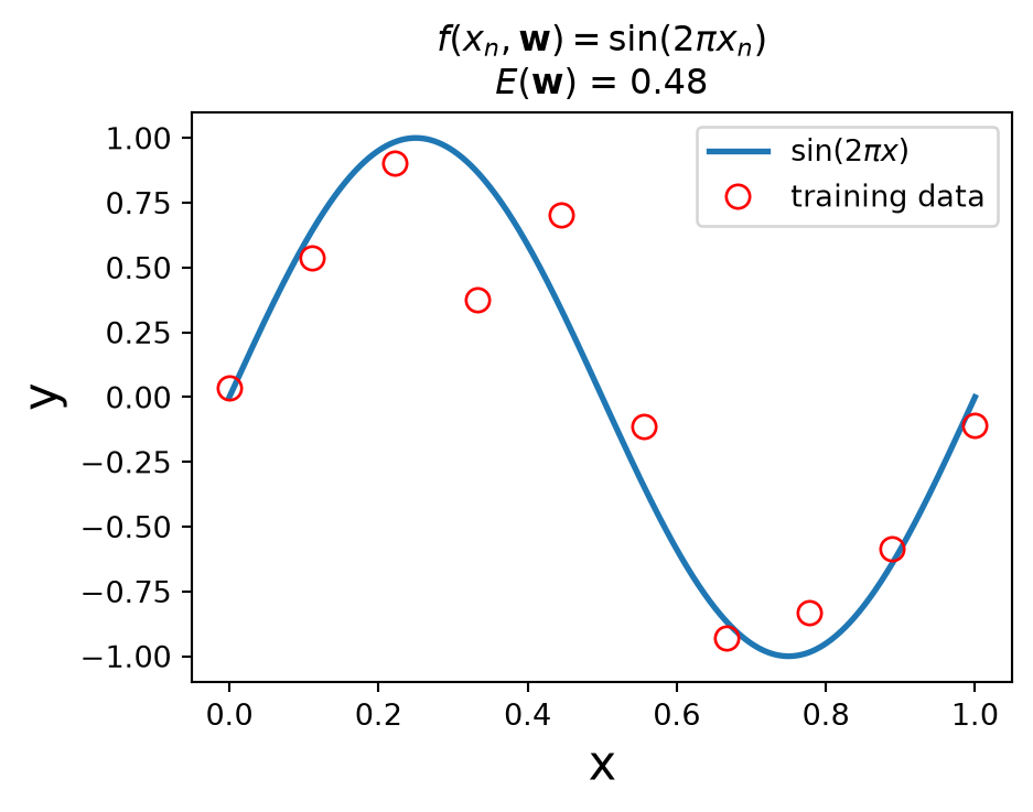
We generate \(N = 10\) points \(x_i\) equally spaced in \([0, 1]\), and set

\[ y_i = \sin(2\pi x_i) + \epsilon_i, \]

where \(\epsilon_i\) is Gaussian noise.

Many data sets are like this: some component of \(y\) depends on \(x\), and some component we treat as random – “noise” – because it depends on features we cannot see.

We will fit polynomials of order \(k\),

\[ f(x, \mathbf{w}) = \sum_{j = 0}^k w_jx^j, \]

choosing \(\mathbf{w}\) to minimize the least squares training error \(E(\mathbf{w}) = \sum_{n=1}^N [f(x_n, \mathbf{w}) - y_n]^2\).

(How to solve for \(\mathbf{w}\) is the subject of Linear Regression.)

Code

N = 10
x = np.linspace(0, 1, N)
from numpy.random import default_rng
y = np.sin(2 * np.pi * x) + default_rng(2).normal(size = N, scale = 0.20)
cx = np.linspace(0, 1, 1000)
cy = np.sin(2 * np.pi * cx)
E_true = np.sum((np.sin(2 * np.pi * x) - y)**2)
plt.figure(figsize = (5, 3.5))
plt.plot(cx, cy, lw = 2, label = r'$\sin(2\pi x)$')
plt.plot(x, y, 'ro', markersize = 8, fillstyle = 'none', label = 'training data')
plt.title(r'$f(x_n, \mathbf{w}) = \sin(2\pi x_n)$' + '\n' + r'$E(\mathbf{w})$ =' + ' {:0.2f}'.format(E_true))
plt.xlabel('x', size = 16)
plt.ylabel('y', size = 16)
plt.legend(loc = 'best');

Model Selection

\(\mathbf{w} = (w_0, \dots, w_k)\) are the parameters of the model; least squares finds the \(\mathbf{w}^*\) that minimizes the error on the training data.
But what about choosing \(k\), the order of the polynomial?
A cubic (\(k = 3\)) is a different model from a quadratic (\(k = 2\)). The problem of choosing \(k\) is called model selection.

Model Selection, cont.

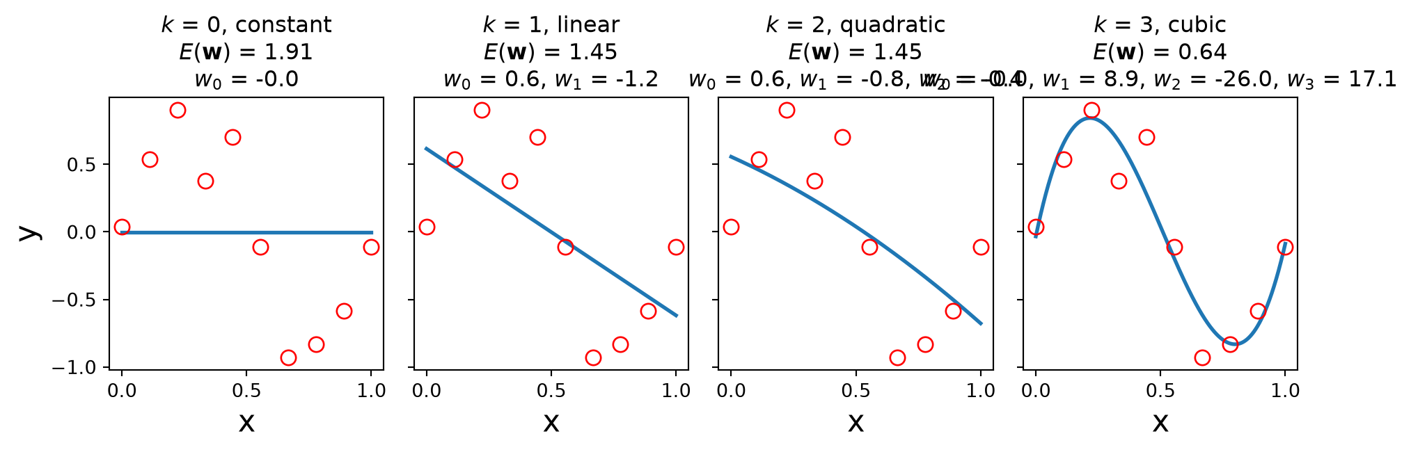
Let’s look at constant (order 0), linear (order 1), and cubic (order 3) models, each fit using the least squares criterion:

Code

# y = Aw, A is design matrix 1, [1, x^T], [1, x^T, x^T^2], etc, and w-hat = (A^TA)^-1 A^Ty
import warnings
warnings.filterwarnings('ignore')

def design_matrix(x, k):
    """Return the N x (k+1) matrix whose columns are 1, x, x^2, ..., x^k."""
    N = len(x)
    A = np.ones(N)
    for i in range(1, k+1):
        A = np.column_stack([A, (x.T)**i])
    return A

def fit_poly(x, y, k):
    """Least-squares weights w_0, ..., w_k of a degree-k polynomial fit to (x, y)."""
    A = design_matrix(x, k)
    w_hat = np.linalg.inv(A.T @ A) @ A.T @ y
    return w_hat

w_hat_0 = 1/N * np.sum(y)
w_hat_1 = fit_poly(x, y, 1)
w_hat_2 = fit_poly(x, y, 2)
w_hat_3 = fit_poly(x, y, 3)

So it looks like a third-order polynomial (\(k\) = 3) is a good fit!

How do we know it’s good? Well, the training error \(E(\mathbf{w})\) is small.

Make training error smaller?

Yes, we can, if we increase the order of the polynomial.

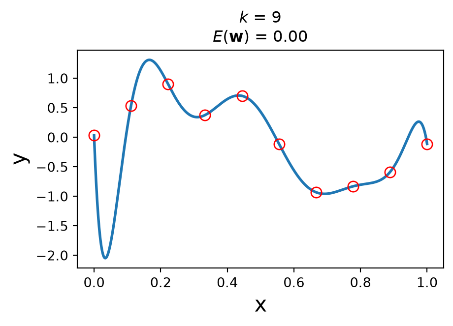
We can reduce the error to zero by setting \(k = 9\), we get the following polynomial fit to the data:

Code

w_hat_9 = fit_poly(x, y, 9)
cy = design_matrix(cx, 9) @ w_hat_9
plt.figure(figsize = (5, 3))
plt.plot(cx, cy, lw = 2, label = r'$k$ = 9')
plt.plot(x, y, 'ro', markersize = 8, fillstyle = 'none')
plt.xlabel('x', size = 16)
plt.ylabel('y', size = 16)
plt.title(r'$k$ = 9' + '\n' + r'$E(\mathbf{w})$ =' + ' {:0.2f}'.format(0));

So … is the 9th order polynomial a “better” model for this dataset?

Absolutely not!

Why?

Informally, the model is very “wiggly”. It seems unlikely that the real data generation process is governed by this curve.
In other words, we don’t expect that, if we had more data from the same source, that this model would do a good job of fitting the additional data.
We want the model to do a good job of predicting on future data.
This is called the model’s generalization ability.

The 9th degree polynomial would seem to have poor generalization ability.

Generalization Error

To assess generalization, we evaluate each polynomial on new test data – not part of the training set.
- We can only do this because we know the generator and can make fresh data. With real data the test set has to come from a split, and we will see that this matters.
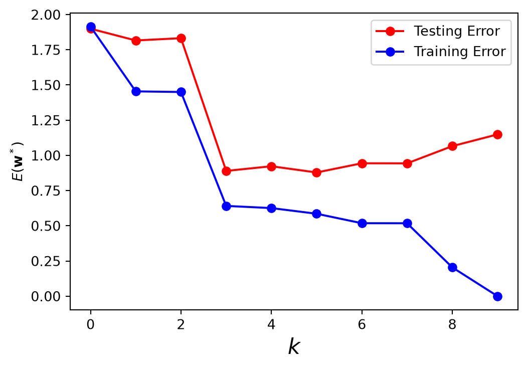
As we increase the order of the polynomial, the training error always declines.
Eventually, the training error reaches zero.
However, the test error does not – it reaches its smallest value at \(k = 3\), a cubic polynomial.
The phenomenon in which training error declines, but testing error does not, is called overfitting.
In a sense we are fitting the training data “too well”.

Code

test_y = np.sin(2 * np.pi * x) + default_rng(8).normal(size = N, scale = 0.20)
max_k = N
train_err = [np.linalg.norm(y - N * [w_hat_0])]
test_err = [np.linalg.norm(test_y - N * [w_hat_0])]
for k in range(1, max_k):
    w_hat = fit_poly(x, y, k)
    pred_y = design_matrix(x, k) @ w_hat
    train_err.append(np.linalg.norm(y - pred_y))
    test_err.append(np.linalg.norm(test_y - pred_y))
plt.figure(figsize = (6, 4))
plt.plot(range(max_k), test_err, 'ro-', label = 'Testing Error')
plt.plot(range(max_k), train_err, 'bo-', label = 'Training Error')
plt.xlabel(r'$k$', size = 16)
plt.ylabel(r'$E(\mathbf{w}^*)$')
plt.legend(loc = 'best');

Overfitting

There are two ways to think about overfitting:

The number of parameters in the model is too large, compared to the size of the training data. We can see this in the fact that we have only 10 training points, and the 9th order polynomial has 10 coefficents.
The model is more complex than the actual phenomenon being modeled. As a result, the model is not just fitting the underlying phenomenon, but also the noise in the data.

These suggest techniques we may use to avoid overfitting:

Increase the amount of training data. All else being equal, more training data is always better.
Limit the complexity of the model. Model complexity is often controlled via hyperparameters.
Use regularization – constrain the model to avoid overfitting.

Bias and Variance

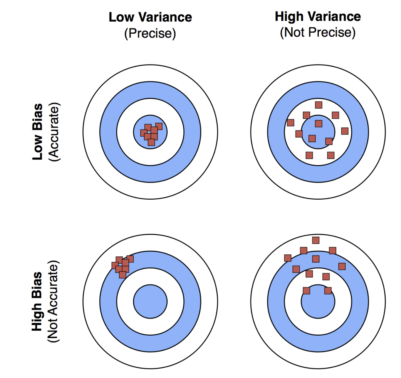
Overfitting is one of two ways a model can be wrong.

Bias

Error due to an overly simplistic model.
High bias: the model underfits – it misses the real pattern. (Our \(k = 0\) or \(k = 1\) polynomial.)
Low bias: the model is flexible enough to capture the underlying pattern.

Variance

Error due to an overly complex model.
High variance: the model overfits – refit it on a different training sample from the same distribution and you get a very different answer. (Our \(k = 9\) polynomial.)
Low variance: predictions are stable across different training sets.

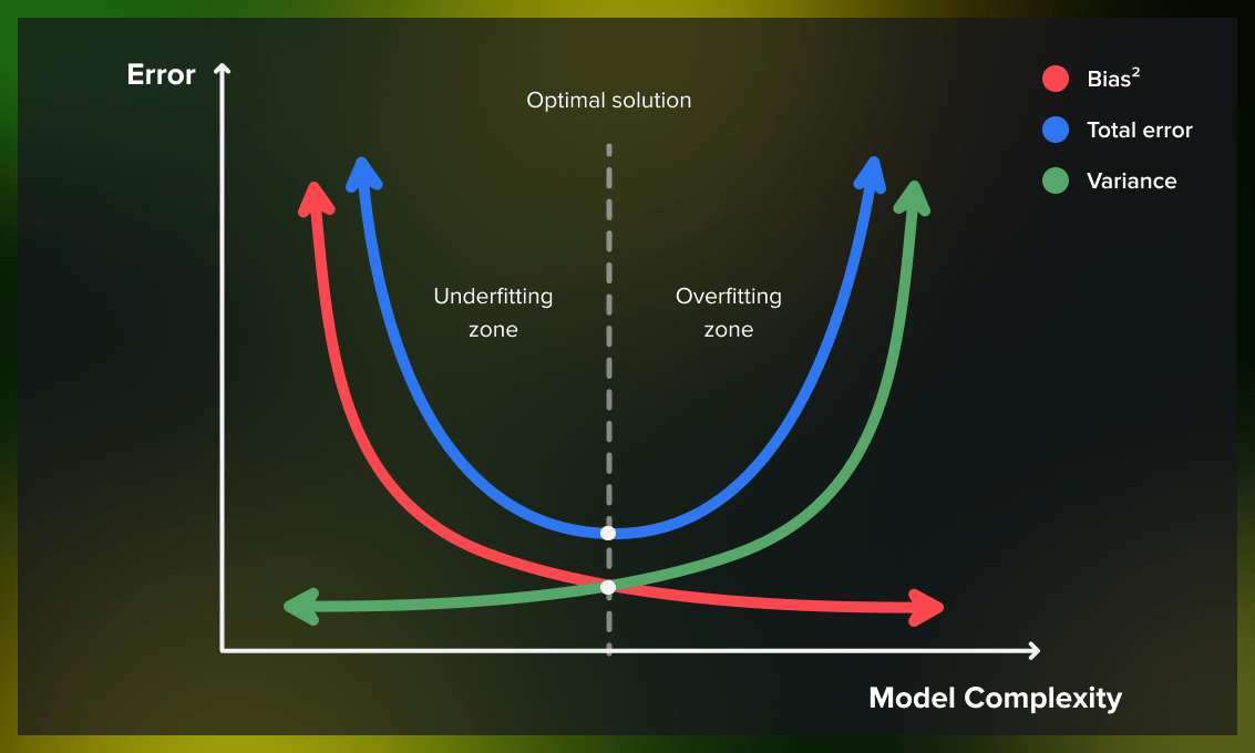
Bias-Variance Trade-Off

Goal: find the model complexity that minimizes total error.

Low bias and low variance are both ideal, but hard to achieve simultaneously: making a model more flexible lowers bias and raises variance.
The U-shaped test error curve we just saw is this trade-off in action – \(k = 3\) is the sweet spot.

Parameters and Hyperparameters

Notice that the model selection problem required us to choose a value \(k\) that specifies the order of the polynomial model.
The values \(w_0, w_1, \dots, w_k\) are the parameters of the model; they are learned from the training data.
In contrast, \(k\) is called a hyperparameter.

A hyperparameter is a parameter that must be set first, before the (regular) parameters can be learned.
Hyperparameters are often used to control model complexity.
So, to avoid overfitting, we need to choose the proper value for the hyperparameter \(k\).
We do that by holding out data.

Holding Out Data

We want to avoid overfitting, which occurs when a model fails to generalize – that is, when it has high error on data that it was not trained on.
So: we will hold some data aside, and not use it for training the model, but instead use it to choose the hyperparameter \(k\).
Let’s assume that we have 20 data points to work with. scikit-learn’s train_test_split() splits them randomly into training and testing sets:

N = 20
x = np.linspace(0, 1, N)
y = np.sin(2 * np.pi * x) + default_rng(2).normal(size = N, scale = 0.20)

import sklearn.model_selection as model_selection

x_train, x_test, y_train, y_test = model_selection.train_test_split(
        x, y, test_size = 0.5, random_state = 0)

print(f'Number of items in training set: {x_train.shape[0]}, in testing set: {x_test.shape[0]}')

Number of items in training set: 10, in testing set: 10

Grid Search

Our strategy will be, for each possible value of the hyperparameter \(k\):

randomly split the data 5 times
fit the model on the training data
test the model on the testing data
compute the mean testing and training error over the 5 random splits

Trying all candidate values of the hyperparameter this way is called a grid search.

(What are good candidate values? It depends on the problem, and may involve trial and error.)

Grid Search, cont.

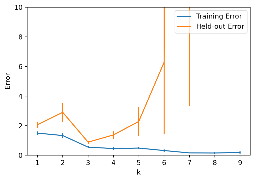
Mean error for each value of k, with its standard error (\(\sigma/\sqrt{n=5}\)) over the 5 splits:

Code

def model_error(x_train, y_train, x_test, y_test, k):
    '''
    This function fits a polynomial of degree k to the training data
    and returns the error on both the training and test data.
    '''
    w_star = fit_poly(x_train, y_train, k)
    pred_test_y = design_matrix(x_test, k) @ w_star
    pred_train_y = design_matrix(x_train, k) @ w_star
    return (np.linalg.norm(y_train - pred_train_y), np.linalg.norm(y_test - pred_test_y))

np.random.seed(7)
max_k = 10
n_splits = 5
err = []
for k in range(1, max_k):
    for s in range(n_splits):
        x_train, x_test, y_train, y_test = model_selection.train_test_split(
            x, y, test_size = 0.5)
        split_train_err, split_test_err = model_error(x_train, y_train, x_test, y_test, k)
        err.append([k, s, split_train_err, split_test_err])
df = pd.DataFrame(err, columns = ['k', 'split', 'Training Error', 'Held-out Error'])

df.groupby('k').mean()[['Training Error', 'Held-out Error']].plot(
    yerr = df.groupby('k').std()/np.sqrt(n_splits), figsize = (6, 4))
plt.ylabel('Error')
plt.ylim([0, 10]);

From this plot we can conclude that, for this dataset, a polynomial of degree \(k = 3\) has the lowest error on the held-out splits, so \(k = 3\) is the value to choose.

Wait: Which Set Did We Just Use to Choose \(k\)?

We held data out “to test generalization.” Then we used it to choose \(k\).
The chosen \(k\) is the best of nine noisy scores, so that score is optimistic. It is no longer an estimate of how the model will do on new data.
Name the roles. Data held out from training to choose hyperparameters is the validation set. Data you never touch during selection is the test set. Everything on the last two slides was validation.
The discipline: split off the test set once, first, and lock it away. Do all selection with train/validation splits inside what remains. Refit the chosen model on all the training data. Evaluate on the test set once, and report that number.
\(k = 3\) is still the right choice. What we don’t yet have is an honest number for how well it generalizes.

Hold Out Strategies

Deciding how much, and which, data to hold out depends on a number of factors.
In general we’d like to give the training stage as much data as possible to work with.
However, the more data we use for training, the less we have for testing – which can decrease the accuracy of the testing stage.
Furthermore, any single partition of the data can introduce dependencies – any class that is overrepresented in the training data will be underrepresented in the test data.

There are two ways to address these problems:

Random subsampling: partition the data randomly between train and test sets, and repeat a reasonable number of times (usually five at least). This is what we just did with train_test_split().
\(K\)-Fold Cross-validation

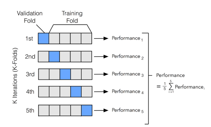
\(K\)-Fold Cross-Validation

In \(K\)-Fold Cross-validation, the data is partitioned once, and then each partition is used as the validation data once.

This ensures that all the data gets equal weight in the training and in the validation.

We divide the data into \(k\) “folds”.
The value of \(k\) can vary up to the size of the dataset.
The larger \(k\) we use, the more data is used for training, but the more folds must be evaluated, which increases the time required.
In the extreme case where \(k\) is equal to the data size, then each data item is held out by itself; this is called “leave-one-out”.

Every Look at the Test Set Spends It

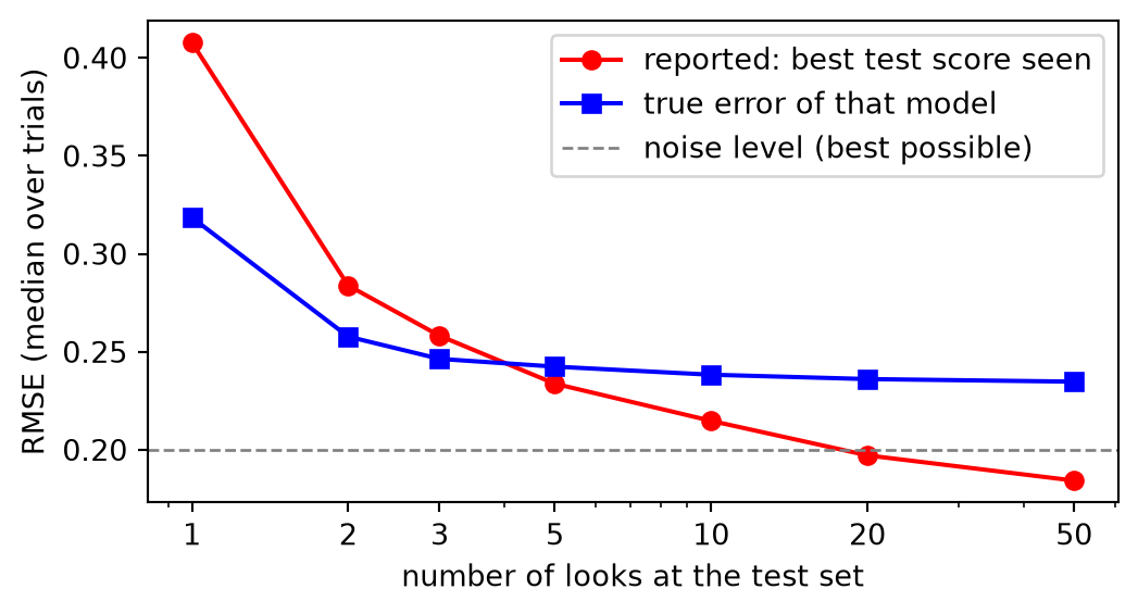
A simulation of an analyst who keeps going back to the test set. The setup:

Start with our usual 20 points. Split them once: 14 for training, 6 locked away as the test set.
The analyst tries \(m\) variants of the model. Here a variant is a polynomial of degree 1 to 5, fitted on a random 11 of the 14 training points – a stand-in for the tweaks people actually make: a different degree, a different feature set, a different subsample.
Each variant is scored on the 6 test points. The analyst keeps whichever variant scored best and reports that score. That is the “look”: the test set has been used to make a decision.
To judge the report, we also compute each variant’s true error on 2,000 freshly generated points. We can only do this because our data is synthetic and we know the generator, \(\sin(2\pi x)\) plus noise. With real data this quantity is exactly the thing you never get to see – which is the whole point.
Repeat the experiment 1,000 times with fresh data, and plot the median reported score and the median true error against the number of looks \(m\).

Code

def rmse(y, pred):
    """Root-mean-square error: comparable across sets of different sizes, unlike the norm used above."""
    return np.sqrt(np.mean((y - pred)**2))

rng = default_rng(3)
looks = [1, 2, 3, 5, 10, 20, 50]              # how many variants the analyst has scored on the test set
n_trials, n_test, n_variants = 1000, 6, 50    # repeat the whole experiment 1000 times; 6 test points; up to 50 looks
reported = {m: [] for m in looks}             # the score the analyst reports after m looks
true_err = {m: [] for m in looks}             # the true error of the model behind that report

for _ in range(n_trials):
    # A fresh sample of 20 points from the same generator as before.
    y_all = np.sin(2 * np.pi * x) + rng.normal(size = N, scale = 0.20)

    # Split ONCE: 14 training points, 6 test points that the analyst may only score against.
    idx = rng.permutation(N)
    x_tr, y_tr = x[idx[n_test:]], y_all[idx[n_test:]]
    x_te, y_te = x[idx[:n_test]], y_all[idx[:n_test]]

    # The TRUE error of a model is its error on new data from the same source. We can measure it
    # only because we know the generator; 2000 fresh points make the estimate essentially exact.
    # No real-data project can compute this line.
    x_fresh = rng.uniform(0, 1, 2000)
    y_fresh = np.sin(2 * np.pi * x_fresh) + rng.normal(size = 2000, scale = 0.20)

    # The analyst's variants. Each row: (score on the 6 test points, true error on the fresh points).
    scores = []
    for _ in range(n_variants):
        k = rng.integers(1, 6)                                # a degree from 1 to 5 ...
        sub = rng.choice(len(x_tr), 11, replace = False)      # ... fitted on a random 11 of the 14 training points
        w = fit_poly(x_tr[sub], y_tr[sub], k)
        test_score = rmse(y_te, design_matrix(x_te, k) @ w)
        true_score = rmse(y_fresh, design_matrix(x_fresh, k) @ w)
        scores.append((test_score, true_score))
    scores = np.array(scores)

    # After m looks the analyst has seen the first m test scores and keeps the best one.
    # We record the score they would report, and the true error of that same model.
    for m in looks:
        best = np.argmin(scores[:m, 0])
        reported[m].append(scores[best, 0])
        true_err[m].append(scores[best, 1])

Every Look at the Test Set Spends It, cont.

Code

plt.figure(figsize = (6, 3))
plt.plot(looks, [np.median(reported[m]) for m in looks], 'ro-', label = 'reported: best test score seen')
plt.plot(looks, [np.median(true_err[m]) for m in looks], 'bs-', label = 'true error of that model')
plt.axhline(0.20, color = 'gray', ls = '--', lw = 1, label = 'noise level (best possible)')
plt.xscale('log'); plt.xticks(looks, looks)
plt.xlabel('number of looks at the test set'); plt.ylabel('RMSE (median over trials)')
plt.legend(loc = 'upper right');

The first few looks improve the model: picking the best of a handful of variants is real selection, and the true error (blue) drops.
After about five looks the true error stops falling. The reported score (red) keeps falling anyway – by twenty looks it is below the noise level, a value no real model can achieve. From there on, only the number improves.
After you have looked, the test set is a validation set: its score is optimistic, and you cannot un-look.
“I’ll go back and retrain after the final evaluation” is the same mistake in slow motion. Iterate inside train/validation. If you must revisit after the test, get fresh test data, or report the score as what it now is: a validation score.
This is why Kaggle scores a hidden private leaderboard: competitors overfit the public one by exactly this mechanism.

How This Plays Out This Term

Every supervised lecture returns to today’s ideas – the same trade-off, a different knob:

Decision Trees: overfit via depth; random forests reduce variance by averaging.
\(k\)-NN: choosing \(k\) – small \(k\) overfits, large \(k\) underfits.
Regression: regularization penalizes complexity directly.
Neural Networks: early stopping – halt training when held-out error starts to rise.

In every case, the hyperparameter is chosen by cross-validation, never by training error, and never by the test set.

Conclusions

We have seen strategies that allow us to learn from data:

Define a set of possible models
Define an error function that tells us when the model is predicting well
Using the error function, search through the space of models to find the best performer

We’ve also seen that there are some subtleties to this approach that must be dealt with to avoid problems:

Simply using the model that has lowest error on the training data will overfit.
Overfitting (variance) and underfitting (bias) are the two ways a model can be wrong; the goal is to balance them.
We need to hold out data to assess the generalization ability of each trained model.
We control model complexity using hyperparameters.
We choose the best hyperparameters based on performance on held-out validation data, and report generalization on a test set that we look at once.

Generalization: Why Training Error Lies

Introduction

The Supervised Learning Problem

The Supervised Contract

A Toy Example1: Polynomial Curve Fitting

Model Selection

Model Selection, cont.

Make training error smaller?

Absolutely not!

Generalization Error

Overfitting

Bias and Variance

Bias-Variance Trade-Off

Parameters and Hyperparameters

Holding Out Data

Grid Search

Grid Search, cont.

Wait: Which Set Did We Just Use to Choose \(k\)?

Hold Out Strategies

\(K\)-Fold Cross-Validation

Every Look at the Test Set Spends It

Every Look at the Test Set Spends It, cont.

How This Plays Out This Term

Conclusions

A Toy Example¹: Polynomial Curve Fitting