Recap: \(k\)-Nearest Neighbors, the Curse of Dimensionality, and Naive Bayes
DS701 Session 11 — Tue Oct 13, 2026 (Monday schedule)
The data is the model
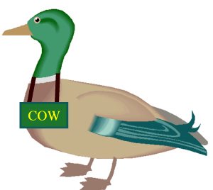
walks like a duck, quacks like a duck…
- Train: store the points. That’s it.
- Predict: distances → \(k\) closest → vote (hard) or vote fractions (soft)
- Nonparametric: the training set is the parameters
- Cost moves to test time: \(O(n)\) distances per prediction
- Scale your features — or one large-unit column picks the neighbours
\(k\) is the bias–variance knob
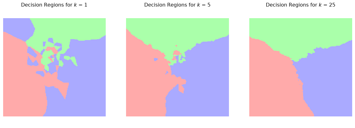
- \(k=1\): islands, 100% train accuracy — low bias, high variance
- \(k=25\): smooth regions — low variance, more bias
- Choose \(k\) on held-out data, never training error (lecture 07)
Choosing \(k\)
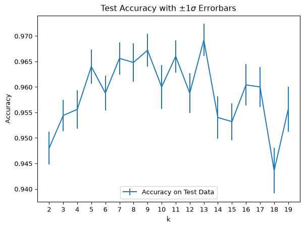
- Iris, mean of 50 random splits per \(k\)
- Peak at \(k = 13\), but error bars overlap 9–13
- One split = one noisy sample → average many, or use \(K\)-fold CV
- Tune on validation; touch test once
The curse, part 1: space explodes
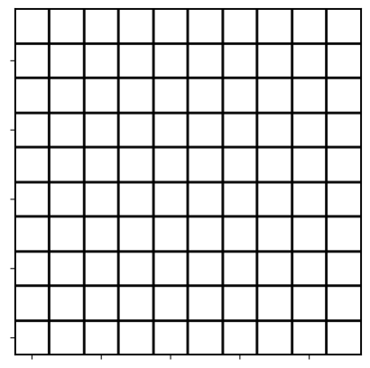
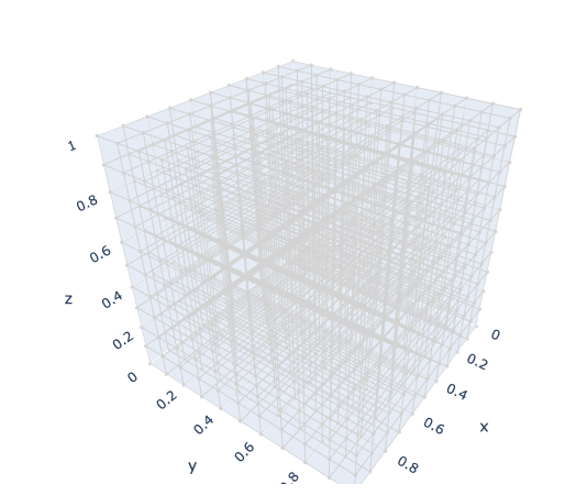
- \(k\)-NN needs dense data
- 10 bins × 40 features = \(10^{40}\) bins — nearly all empty
- Close in \(\mathbb{R}^d\) = close in every coordinate
- Data needed grows exponentially in \(d\)
The curse, part 2: “nearest” fades
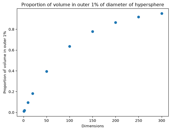

- Every neighbour is about equally far → \(k\) “nearest” ≈ random
- Fixes: other metrics (cosine), or reduce dimension (lectures 12–13)
The naive assumption — and why it works
\[ P(x_1,\dots,x_d \mid C_i) = \prod_{j=1}^{d} P(x_j \mid C_i) \]
- \(10^{20}\) bins → \(20 \times 10\); training = counting
- Rarely true, but only the arg max must be right
- No distances → high \(d\) isn’t the same enemy
- One empty bin zeroes the product → Laplace smoothing

Logistics
- Groups of 2–3 — open your section’s notebook
- (autograded) parts → Gradescope; the rest is participation
- Staff will circulate — be ready to explain your work


Goes live on lecture day. Colab optional — or run locally from GitHub.