Recap: Logistic Regression and Regularization
DS701 Session 13 — Mon Oct 19, 2026
Logistic regression = a linear model + a sigmoid
Last week: a continuous \(y\) as a linear function of \(x\). This week: a 0/1 \(y\), and we want a probability.
- A line takes values in \((-\infty,\infty)\); a probability lives in \([0,1]\). So fit the line to something unbounded: the log-odds \(\log\frac{p}{1-p}\) (the logit).
- Invert: \(p(x) = \sigma(\beta_0 + \beta_1 x)\), the sigmoid.
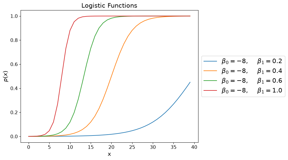
- \(\beta_1\) sets the steepness (and direction); \(\beta_0\) shifts the curve; \(p = 0.5\) at \(x = -\beta_0/\beta_1\); \(\beta_0\) alone is the base rate.
- Read a coefficient exactly as in linear regression — but on the log-odds scale.
Evaluation beyond accuracy: the threshold is a decision
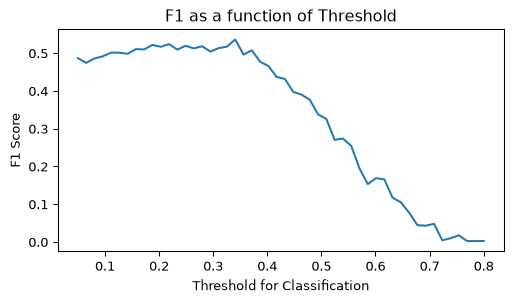
Admissions: F1 peaks near \(t \approx 0.3\) — the model rarely says “admit” at 0.5 because admits are the minority.
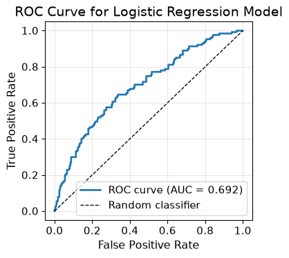
ROC: TPR vs FPR, one point per threshold; diagonal = random; AUC summarizes ranking quality without choosing a threshold (0.69 here).
AUC tells you how good the scores are. It does not tell you where to cut — that depends on the costs of FN vs FP and on the base rate. Today’s stretch: a dataset where 95% accuracy is worthless.
Regularization: a penalty that trades bias for variance
Lecture 07: flexible fits chase noise → high variance. Regularization is the knob:
\[\min_{\boldsymbol{\beta}} \Vert X\boldsymbol{\beta} - \mathbf{y}\Vert_2^2 + c\,R(\boldsymbol{\beta})\]
- Ridge: \(R = \Vert\boldsymbol{\beta}\Vert_2^2\), closed form \((X^\top X + cI)^{-1}X^\top\mathbf{y}\) — always exists, always unique, even with multicollinearity.
- LASSO: \(R = \Vert\boldsymbol{\beta}\Vert_1\).
- \(c = 0\): least squares. \(c \to \infty\): \(\boldsymbol{\beta} \to 0\). In between: fit vs. size — bias bought, variance sold.
- Multicollinearity is the classic reason: nearly dependent columns ⇒ huge \(\kappa(X) = \sigma_{\max}/\sigma_{\min}\) ⇒ wildly unstable \(\hat{\boldsymbol{\beta}}\) (Longley: \(\kappa \approx 10^8\)).
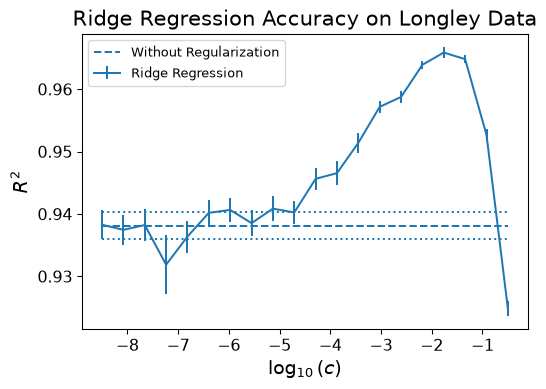
Longley, ridge: held-out \(R^2\) rises with \(c\), then collapses — the sweet spot is found by cross-validation.
\(\ell_2\) shrinks, \(\ell_1\) selects
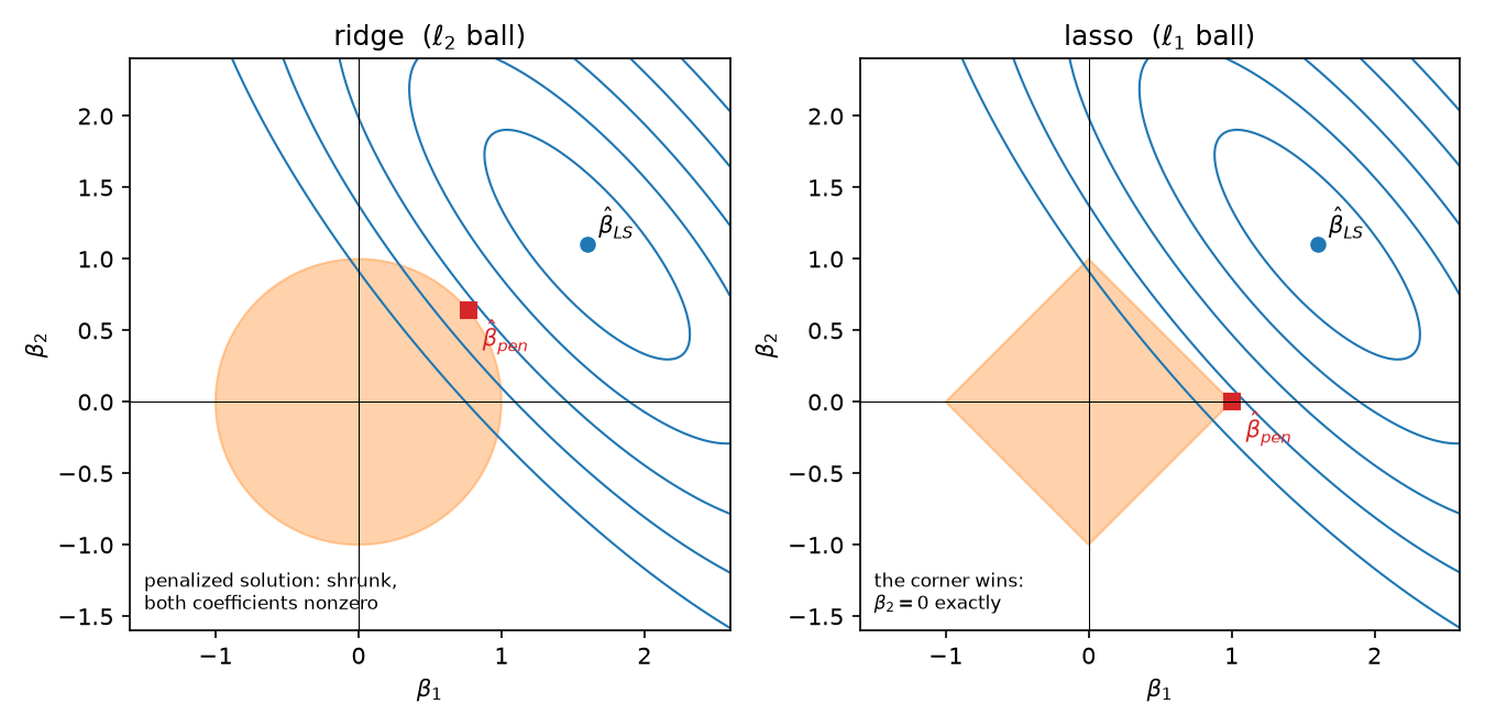
Same contours, different penalty balls. The \(\ell_1\) diamond has corners on the axes — the contours usually hit a corner first, and a corner means a coefficient is exactly zero.
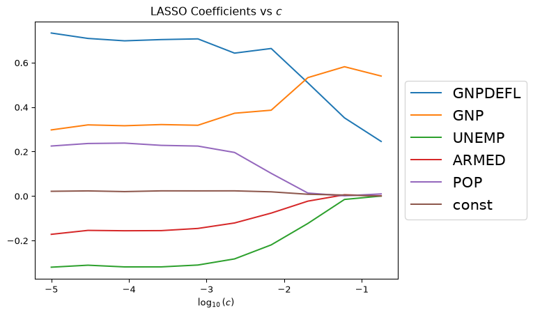
Longley, LASSO: as \(c\) grows, ARMED, UNEMP, POP go to zero; GNP and GNPDEFL remain — the near-dependent variables are the ones dropped.
Ridge never zeroes anything (until \(c \to \infty\), all at once). LASSO gives you model selection for free — instead of searching \(2^n - 1\) subsets — at similar prediction error, with a much more interpretable answer.
Activity: from the likelihood to a threshold you would ship
Goal: build logistic regression from its likelihood and check it against sklearn; trace ridge and lasso paths on data with correlated and irrelevant features, pick \(\alpha\) by CV, and see what forgetting to standardize costs; then take a 90/10 (A1) or 95/5 (B1) imbalanced problem, watch accuracy lie, sweep the threshold, plot ROC and precision–recall, choose a threshold for a stated cost, and try class_weight="balanced".
- Work in groups of 2–3. Open your section’s notebook.
- Parts marked (autograded) are submitted to Gradescope; the rest is participation.
- Staff will circulate — be ready to explain any part of your work.
- Dependencies:
numpy,pandas,matplotlib,scikit-learn.
Section A1 

Section B1
The activity notebook goes live on the day of the lecture. Colab is optional — you can also open it on GitHub and run it locally.