Recap: Recommender Systems
DS701 Session 22 — Wed Nov 18, 2026
The user–item matrix — and the hole in it
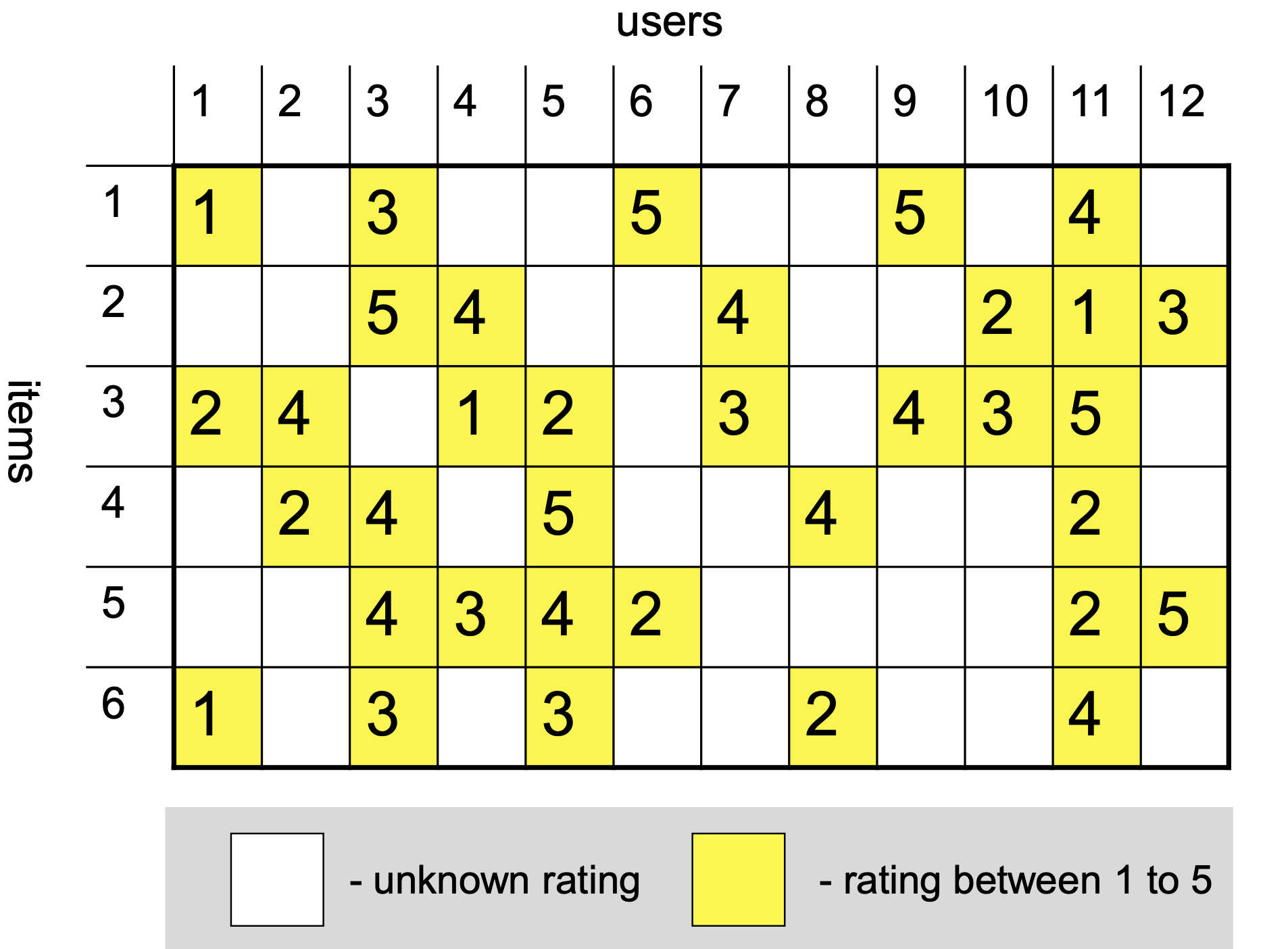
- Rows are items, columns are users, entries are ratings \(r_{ui}\) — the same object as the bipartite graph of known ratings.
- Amazon movies: 1.7M reviews, ~50K movies, ~124K users → 99.97% empty. \[\text{sparsity} = \frac{\#\text{ reviews}}{\#\text{ users}\times\#\text{ items}}\]
- And it is skewed: the average movie has 34 reviews, but most have far fewer (power law) — for most rows there is almost nothing to go on.
- Goal: predict the blanks; score with RMSE on held-out known ratings. Baseline to beat: the global mean \(\mu\).
Collaborative filtering: neighbours in rating space
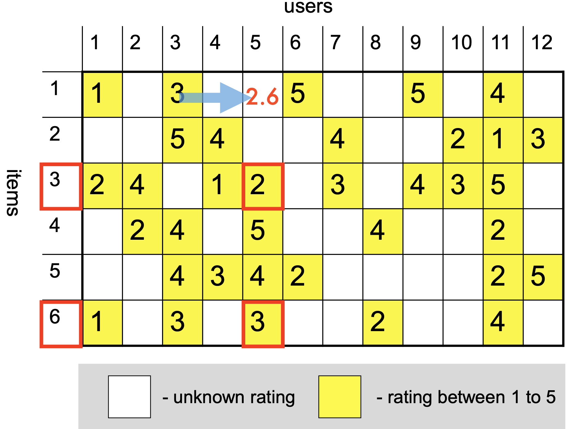
Item–item: to guess \(r_{ui}\), look at items like \(i\) that \(u\) has rated, and average.
\[ \hat r_{ui} = \frac{\sum_{j \in n_k(i,u)} s_{ij}\, r_{uj}}{\sum_{j \in n_k(i,u)} s_{ij}} \qquad \frac{0.84\cdot 2 + 1.0\cdot 3}{0.84 + 1.0} = 2.54 \]
- \(n_k(i,u)\): the \(k\) nearest neighbours of \(i\) among the items \(u\) rated — it is \(k\)-NN.
- \(s_{ij}\): correlation of the two items’ rating rows, over the users who rated both (\(s_{13} = 0.84\), \(s_{16} = 1.0\) in the example).
- User–user is the mirror image. Rule of thumb: compare along the short side — few items, many users → item–item (Netflix; Amazon too): a smaller similarity table, each entry backed by more co-raters.
Matrix factorization: low rank = latent tastes
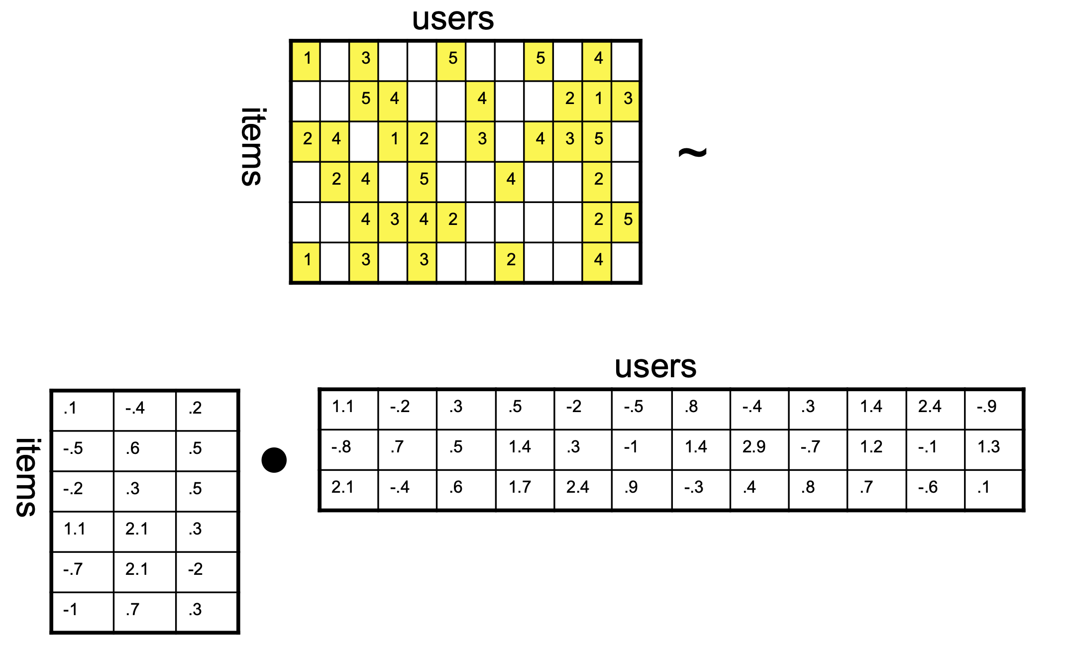
CF uses item similarity or user similarity. MF puts both in one latent space:
- \(R \approx UV^T\) — one \(k\)-vector per user, \(\mathbf u_u\), and per item, \(\mathbf v_i\); predicted rating \(= \mathbf u_u^\top \mathbf v_i\).
- This is Session 14’s SVD picture — rank \(k\) latent factors — but the matrix is partially observed, so we fit only where we can see: \[ \min_{U,V}\ \Vert (R - UV^T)_S\Vert^2 + \lambda\big(\Vert U\Vert^2 + \Vert V\Vert^2\big) \]
- \(\lambda\): ridge penalty — rank 20 with \(\lambda = 1\) reached training RMSE 0.31 but held-out 1.29, worse than the global mean.
Evaluate on ratings you hid
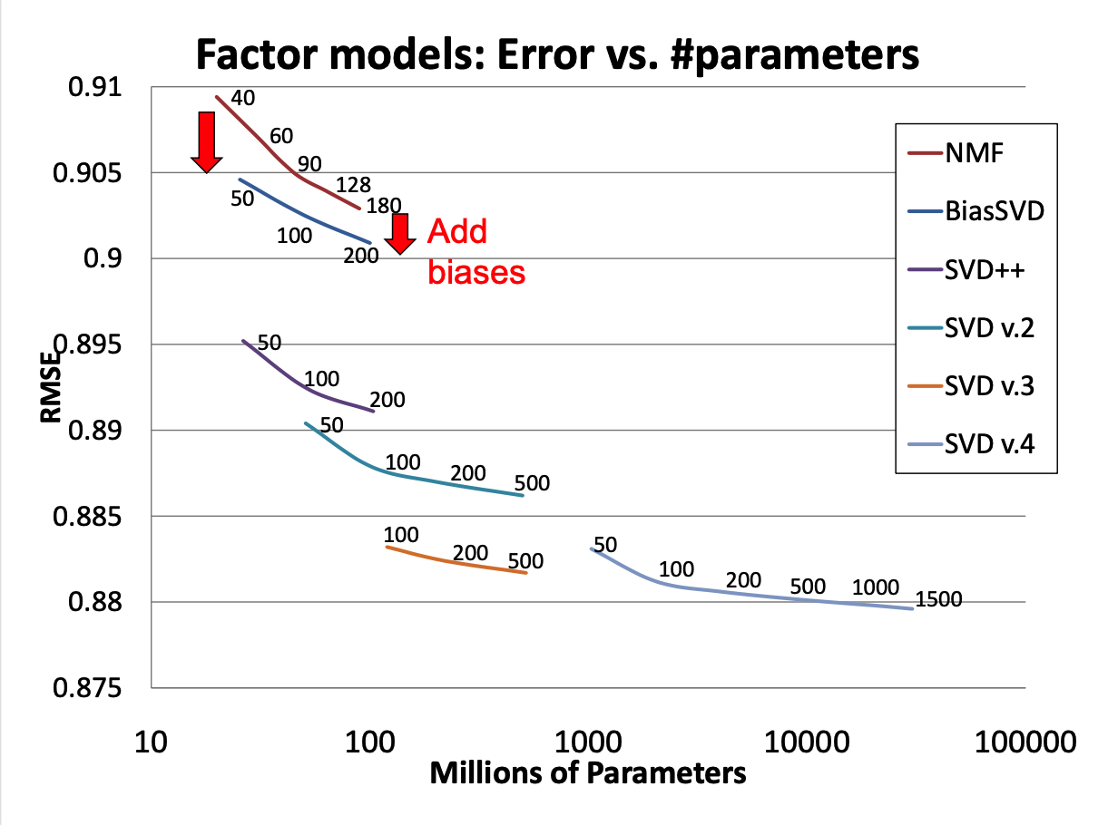
- Honest protocol: hold out a random slice of the known ratings, fit on the rest, predict the slice, RMSE there.
- The lecture’s dense block: global mean 1.17; rank 20, \(\lambda = 1\): 0.31 training but 1.29 held-out; rank 5, \(\lambda = 10\): 1.01. Training RMSE keeps falling with \(k\); held-out RMSE tells you when you are memorising.
- Still optimistic: the densest block, and ratings are missing not at random. The product needs a good top-\(k\) list (precision@\(k\)), and offline ≠ online (A/B test).
- Today: 70% missing, 100 ratings held out, and you will read all three numbers off — global mean, item–item CF, MF.
Activity — Case Study 19: Recommendations for a Public Library’s E-Media Platform
Goal: a public library’s e-media platform wants a “patrons who borrowed this also borrowed…” panel and a plan for brand-new patrons, but its borrowing records cannot leave the library — so you work on a simulator built to the library’s stated shape (80 patrons, 36 titles, planted genres and biases, 70% missing), where the truth is known. Part 1 measures the sparsity and scores two baselines on held-out ratings; Part 2 builds item–item CF by hand (adjusted-cosine similarity, \(k\)-NN prediction) so a librarian can see one recommendation computed; Part 3 implements ALS for matrix factorization, checks it beats the baselines on held-out ratings, and checks the learned factors recover the genres. The report-out answers the library’s second question from the lecture’s cold-start section: what to show a patron who has borrowed nothing.
- Work in groups of 2–3. Open your section’s notebook — the service differs.
- Parts marked (autograded) are submitted to Gradescope; the rest is participation.
- Staff will circulate — be ready to explain any part of your work.
- Dependencies:
numpy,pandas,matplotlib,scikit-learn.


The activity notebook goes live on the day of the lecture. Colab is optional — you can also open it on GitHub and run it locally.