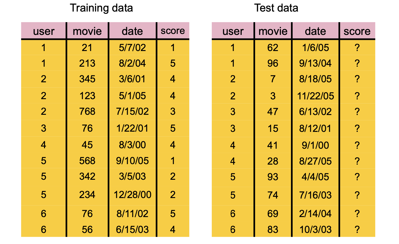
Matrix Factorization Techniques for Recommender Systems, (Koren et al. 2009)
Collaborative Filtering with Temporal Dynamics, (Koren 2009)
What are Recommender Systems?
The concept of recommender systems emerged in the late 1990s / early 2000s as social life moved online:
online purchasing and commerce
online discussions and ratings
social information sharing
In these systems the amount of content was exploding and users were having a hard time finding things they were interested in.
Users wanted recommendations.
Over time, the problem has only gotten worse:
An enormous need has emerged for systems to help sort through products, services, and content items.
This often goes by the term personalization.
Some examples (rough, recent catalogue sizes):
Movie recommendation (Netflix ~6.5K movies and shows, YouTube ~14B videos)
Related product recommendation (Amazon ~600M products)
Web page ranking (Google >>100B pages)
Social content filtering (Facebook, Twitter)
Services (Airbnb, Uber, TripAdvisor)
News content recommendation (Apple News)
Priority inbox & spam filtering (Gmail)
Online dating (Match.com)
A more formal view:
User - requests content
Objects - instances of content
Context - ratings, purchases, views, device, location, time, history
Interface - browser, mobile
Inferring Preferences
Unfortunately, users generally have a hard time explaining what types of content they prefer.
Some early systems worked by interviewing users to ask what they liked. Those systems did not work very well.
Instead, modern systems work by capturing user’s opinions about specific items.
This can be done actively:
When a user is asked to rate a movie, product, or experience,
or it can be done passively:
By noting which items a user chooses to purchase (for example).
Challenges
The biggest issue is scalability: typical data for this problem is huge.
Millions of objects
100s of millions of users
Changing user base
Changing inventory (movies, stories, goods)
Available features
Imbalanced dataset
User activity / item reviews are power law distributed
Example
Let’s look at a dataset for testing recommender systems consisting of Amazon movie reviews.
The full set is 1.7 million reviews with their text (647 MB). We only need two small files derived from it, both in data/amazon-movies/:
review-counts.csv — how many reviews each user wrote and each movie received, stored as a frequency table (kind, reviews, count: “count users wrote exactly reviews reviews”);
dense-block.csv — the (user, movie, star rating) triples we will factor later.
Code
import osDATA ='data/amazon-movies'ifnot os.path.exists(DATA): # e.g. on Colab: read the public copy instead DATA ='https://raw.githubusercontent.com/tools4ds/DS701-Materials-FA26/main/data/amazon-movies'counts = pd.read_csv(f'{DATA}/review-counts.csv')counts.head()
kind
reviews
count
0
item
5
5751
1
item
6
4545
2
item
7
3546
3
item
8
2915
4
item
9
2520
Expanding the frequency table gives one number per user and one per movie:
There are 6,204,445,920 potential reviews, meaning sparsity of 0.0274%
where
\[
\text{sparsity}
= \frac{\text{\# of reviews}}{\text{\# of users} \times \text{\# of movies}}
= \frac{\text{\# of reviews}}{\text{\# of potential reviews}}
\]
Reviews are Sparse
Only about 0.03% of the possible reviews exist – 99.97% of the entries are missing.
Code
display(Markdown(f'There are on average {n_reviews/n_movies:0.1f} reviews per movie'+f' and {n_reviews/n_users:0.1f} reviews per user'))
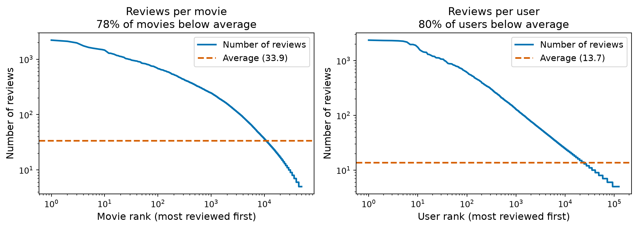
There are on average 33.9 reviews per movie and 13.7 reviews per user
Sparseness is Skewed
Although on average a movie receives 34 reviews and a user writes 14, almost all movies and users have fewer. On log–log axes the users’ rank–frequency curve is close to a straight line, the signature of a power law; the movie curve is heavy-tailed too. (The dataset keeps only users and movies with at least 5 reviews.)
\(r_{ui}\) is the rating that user \(u\) gives to item \(i\), and
\(S\) is the set of (user, item) pairs with a known rating.
The simplest predictor is the global mean, \(\hat r_{ui} = \mu\) for everyone and everything. Every method below must beat its RMSE; we will measure it on held-out ratings at the end.
OK, now we know the problem and the data available. How can we address the problem?
The earliest method developed is called collaborative filtering.
Collaborative Filtering
Collaborative Filtering
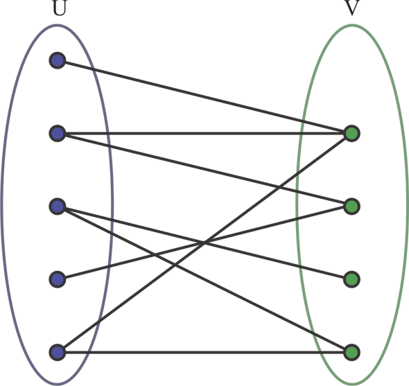
The central idea of collaborative filtering is that the set of known recommendations can be considered to be a bipartite graph.
The nodes of the bipartite graph are users (\(U\)) and items (\(V\)).
Each edge corresponds to a known rating \(r_{ui}.\)
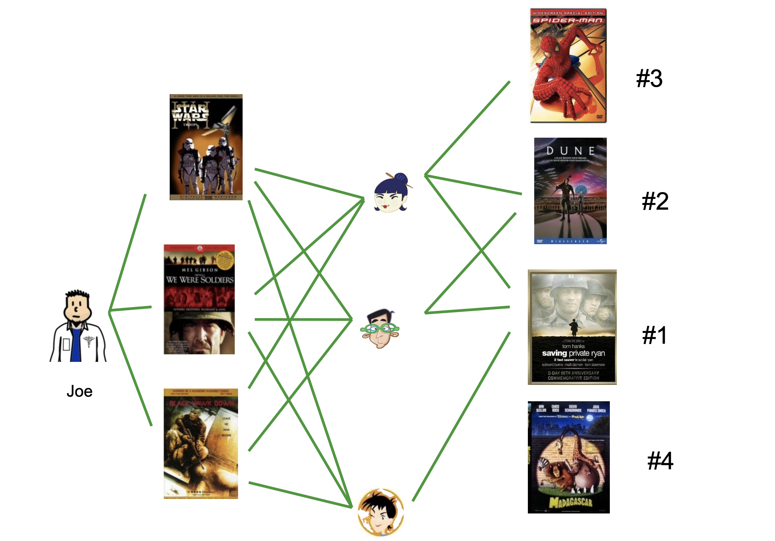
Then recommendations are formed by traversing or processing the bipartite graph.
Joe’s three war films were also watched by two other users. The films they rated highly, ranked by how many of them agree, are Joe’s recommendations.
There are at least two ways this graph can be used.
Two ways to form a rating for the pair \((u, i)\):
Using user-user similarity:
look at users that have similar item preferences to user \(u\)
look at how those users rated item \(i\)
Using item-item similarity:
look at other items that have been liked by similar users as item \(i\)
look at how user \(u\) rated those items
Rule of thumb: compare along the short side of the matrix.
Few items, many users ⟹ item–item (e.g., Netflix: ~6.5K titles, ~280M subscribers).
Few users, many items ⟹ user–user.
Why the short side wins:
Size. With \(m\) items the item–item similarity table has \(m^2\) entries; with \(n\) users the user–user table has \(n^2\). Netflix: \(6{,}500^2 \approx 4\times 10^7\) versus \((2.8\times 10^8)^2 \approx 8\times 10^{16}\).
Support. Each similarity is estimated from the pairs’ co-ratings. Two popular titles share thousands of raters; two random subscribers share a handful of titles.
Stability. Item–item similarities change slowly, so they can be precomputed offline. That is why Amazon, with tens of millions of customers and millions of products, chose item–item as well (Linden et al. 2003; Sarwar et al. 2001).
Item-Item CF
For item-item similarity, we’ll look at item-item Collaborative Filtering (CF).
The questions are:
How do we judge “similarity” of items?
How do we form a predicted rating?
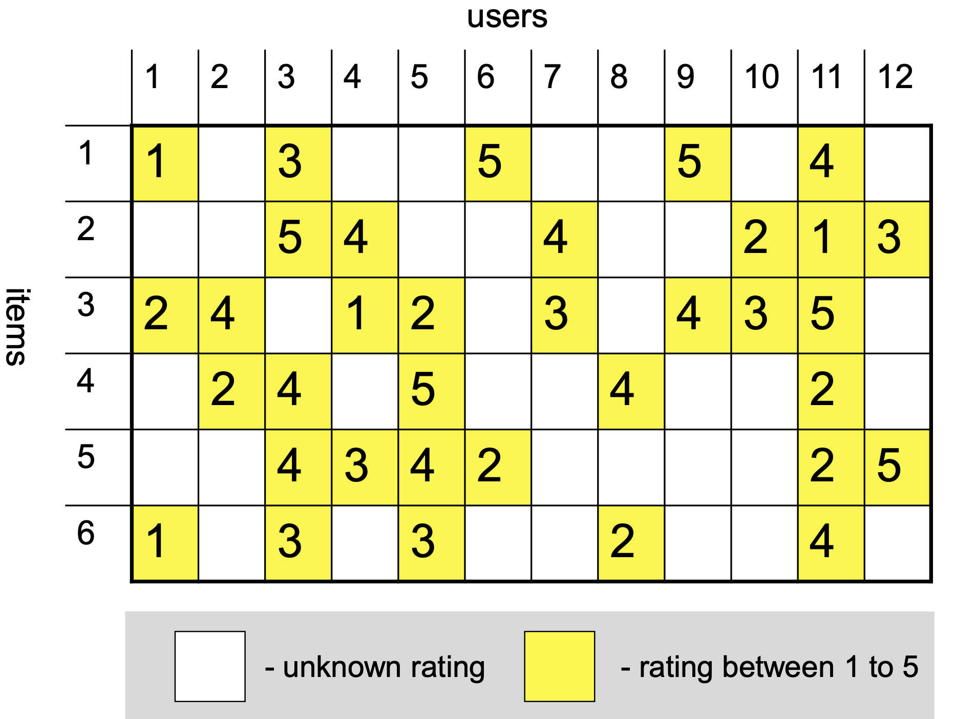
Here is another view of the ratings graph, this time as a matrix that includes missing entries:
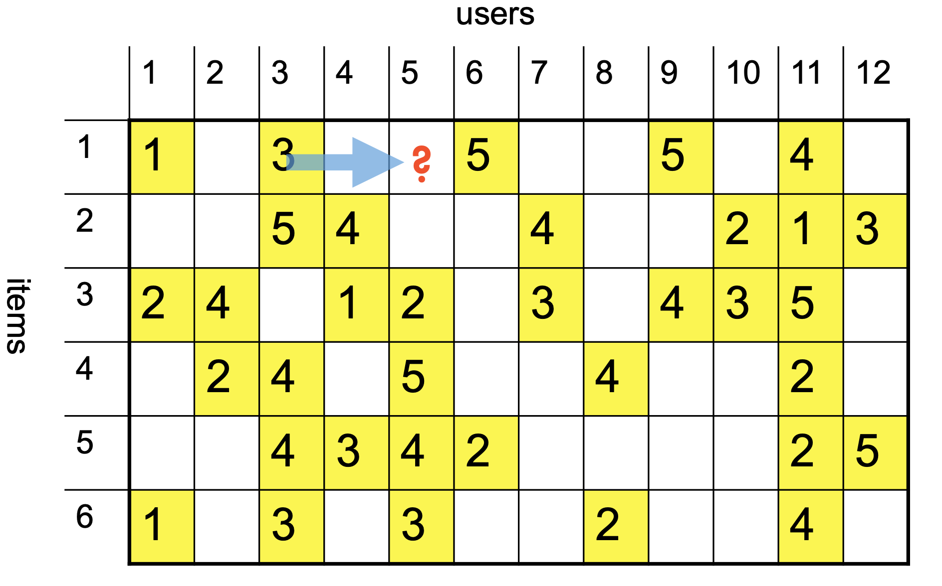
Let’s say we want to predict the value of this unknown rating, user 5’s rating of item 1:
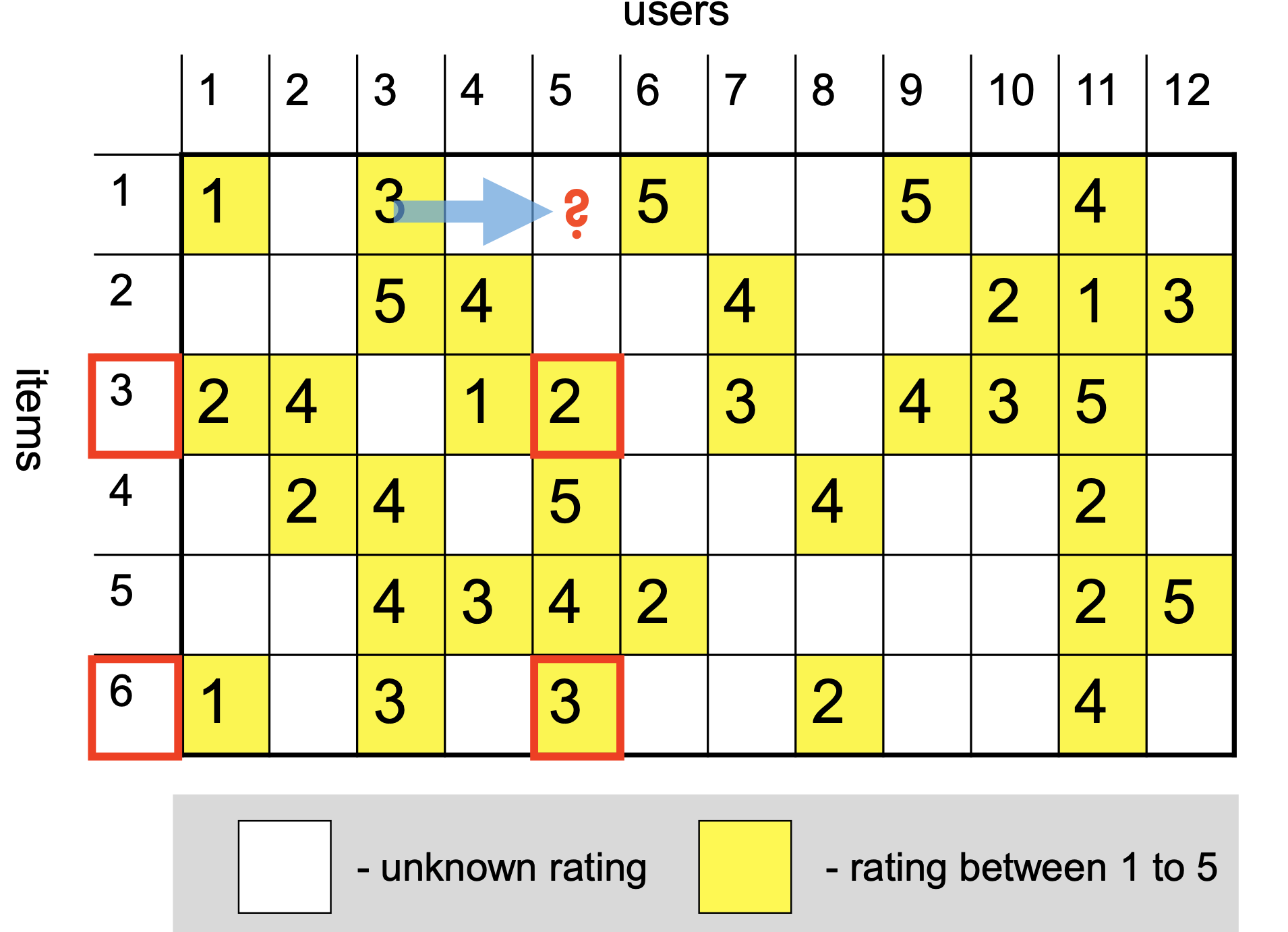
We compare item 1 only with items that user 5 has rated: items 3, 4, 5 and 6.
Similarity \(s_{1j}\) = Pearson correlation of the two item rows, computed over the users who rated both (defined on the next slides):
item \(j\)
co-raters
\(s_{1j}\)
3
users 1, 9, 11
0.84
4
users 3, 11
−1.0
5
users 3, 6, 11
−0.87
6
users 1, 3, 11
1.0
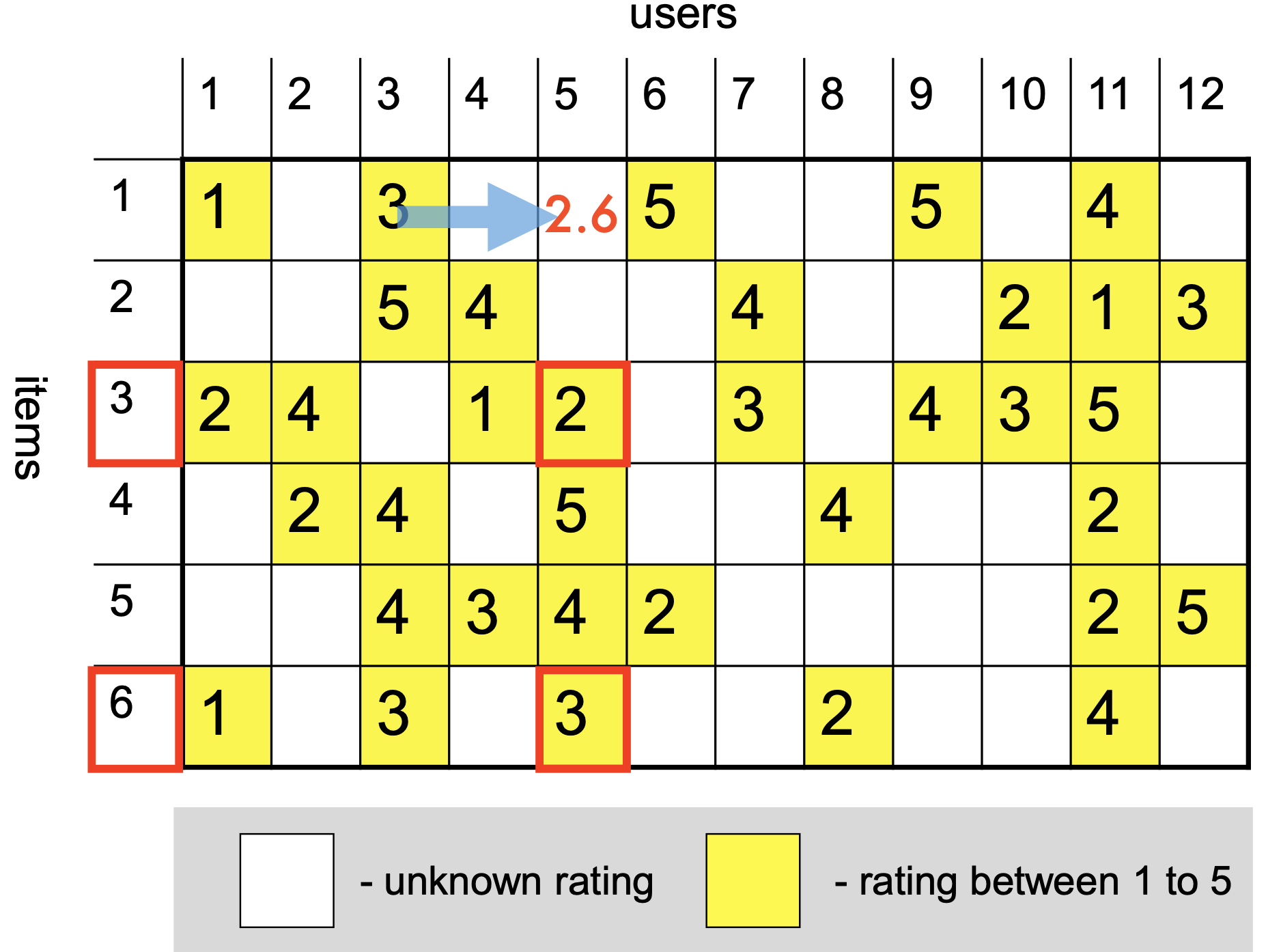
We use \(k\)-nearest neighbors with \(k = 2\): the two most similar, items 3 and 6.
These similarity scores tell us how much weight to put on the rating of the other items.
The user–user mirror on the same matrix: the users who rated item 1 and share at least three items with user 5 (with two, a correlation is always \(\pm 1\), as for item 4 above) are users 3 and 11. User 3 correlates positively (\(0.87\) over items 4, 5, 6) and rated item 1 a 3; user 11 correlates negatively (\(-0.95\)) and is dropped. User–user CF predicts 3.
Similarity
How should we assess similarity of items?
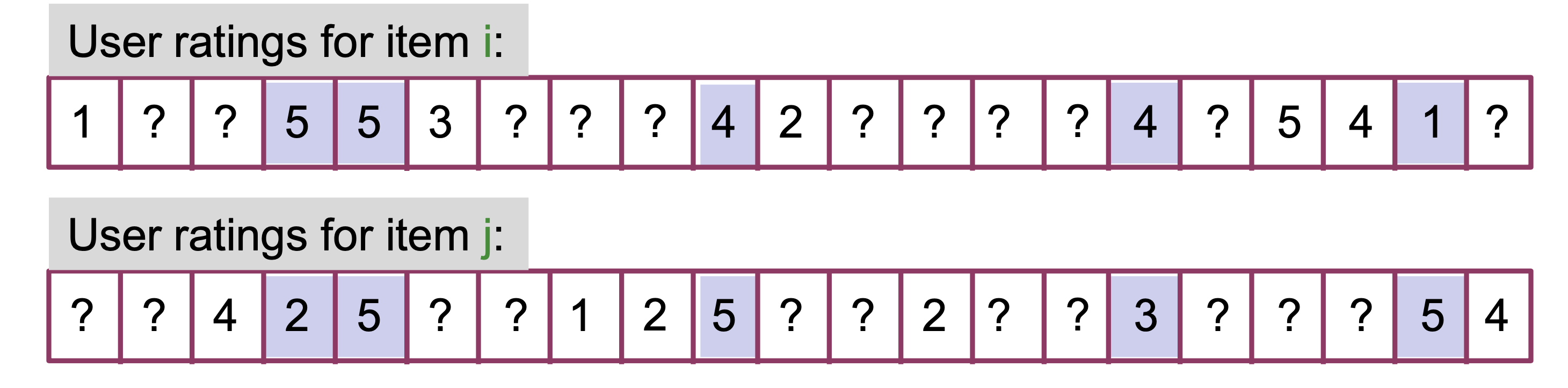
A reasonable approach is to consider items similar if their ratings are correlated, i.e.,
# Keep only the positions where both items have a ratingfiltered_ratings_item_i = [rating_i for rating_i, rating_j inzip(ratings_item_i, ratings_item_j) ifnot np.isnan(rating_i) andnot np.isnan(rating_j)]filtered_ratings_item_j = [rating_j for rating_i, rating_j inzip(ratings_item_i, ratings_item_j) ifnot np.isnan(rating_i) andnot np.isnan(rating_j)]display(Markdown(f'Common ratings for item $i$: {filtered_ratings_item_i}'))display(Markdown(f'Common ratings for item $j$: {filtered_ratings_item_j}'))
Common ratings for item \(i\): [5, 5, 4, 4, 1]
Common ratings for item \(j\): [2, 5, 5, 3, 5]
Example, continued
Code
display(Markdown(f'Common ratings for item $i$: {filtered_ratings_item_i}'))display(Markdown(f'Common ratings for item $j$: {filtered_ratings_item_j}'))
Common ratings for item \(i\): [5, 5, 4, 4, 1]
Common ratings for item \(j\): [2, 5, 5, 3, 5]
Now we can compute the Pearson correlation coefficient:
which (for each column of \(R\)) is a standard regularized least squares problem solved via Ridge regression: \(\hat{\boldsymbol{\beta}} = (X^TX + cI)^{-1}X^T\mathbf{y}\).
Back to Solving the problem
This problem is convex — in fact jointly convex in \(\mu\), \(\alpha\) and \(\beta\), because the prediction is linear in all three: it is one big least-squares problem. Solving for one block at a time is just convenient. (The matrix-factorization problem below is not jointly convex.)
The strategy for solving is:
Hold \(\alpha\) and \(\beta\) constant, solve for \(\mu\).
Hold \(\alpha\) and \(\mu\) constant, solve for \(\beta\).
Hold \(\beta\) and \(\mu\) constant, solve for \(\alpha\).
Each of the three steps will reduce the overall error. As a result, we iterate over them until convergence.
The last issue is that the matrix \(R\) is not dense - in reality we only have a small subset of its entries.
We simply need to adapt the least-squares solution to only consider the entries in \(R\) that we know.
As a result, the actual calculation is as follows…
Here \(i \in R(u)\) means the set of items rated by user \(u\) and \(u \in R(i)\) means the set of users who have rated item \(i\) and \(|R(u)|\) is the number of ratings.
Now that we have learned the biases, we can do a better job of estimating correlation:
When \(s_{ij}\) is negative (negative correlation), here’s what happens:
Numerator: The term \(s_{ij}(r_{uj} - b_{uj})\) becomes negative when \(s_{ij} < 0\). This means:
If user \(u\) rated item \(j\)above its bias (\(r_{uj} - b_{uj} > 0\)), the negative similarity will push the prediction for item \(i\)down
If user \(u\) rated item \(j\)below its bias (\(r_{uj} - b_{uj} < 0\)), the negative similarity will push the prediction for item \(i\)up
This makes intuitive sense: if items \(i\) and \(j\) are negatively correlated, then liking one means you’re likely to dislike the other.
Denominator: When \(s_{ij}\) is negative, it contributes a negative value to the sum in the denominator. This can potentially lead to issues:
If all similarities are negative, the denominator becomes negative
If there’s a mix of positive and negative similarities, they might partially cancel out, potentially making the denominator close to zero or even zero
Common Solutions
To address these issues, practitioners typically use one of these approaches:
Use only positive similarities: Filter out items with negative correlation (only use \(k\)-NN where \(s_{ij} > 0\))
Use absolute values in denominator: \(\displaystyle\hat{r}_{ui} = b_{ui} + \frac{\sum_{j \in n_k(i, u)} s_{ij}(r_{uj} - b_{uj})}{\sum_{j \in n_k(i, u)} |s_{ij}|}\)
The first approach (filtering to positive similarities) is most common because negatively correlated items are typically less informative for prediction than positively correlated items in most domains.
You will sometimes see a third option, rescaling to \([0, 1]\) with \(s'_{ij} = (s_{ij} + 1)/2\). Avoid it: it gives an uncorrelated neighbour weight \(0.5\) and an anti-correlated one weight near \(0\), so it rewards neighbours that carry no information.
Assessing CF
This completes the high level view of CF.
Working with user-user similarities is analogous.
Strengths:
Essentially no training.
The reliance on \(k\)-nearest neighbors helps in this respect.
Easy to update with new users, items, and ratings.
Explainable:
“We recommend Minority Report because you liked Blade Runner and Total Recall.”
Weaknesses:
Accuracy can be a problem – resulting in poor recommendations
Scalability can be a problem – compute grows (think \(k\)-NN)
Matrix Factorization Approaches
Matrix Factorization
Note that standard CF forces us to consider similarity among items, or among users, but does not take into account both.
Can we use both kinds of similarity simultaneously?
We can’t use both the rows and columns of the ratings matrix \(R\) at the same time – the user and item vectors live in different vector spaces.
Now, however, we are working with a matrix which is only partially observed. That is, we only know some of the entries in the ratings matrix.
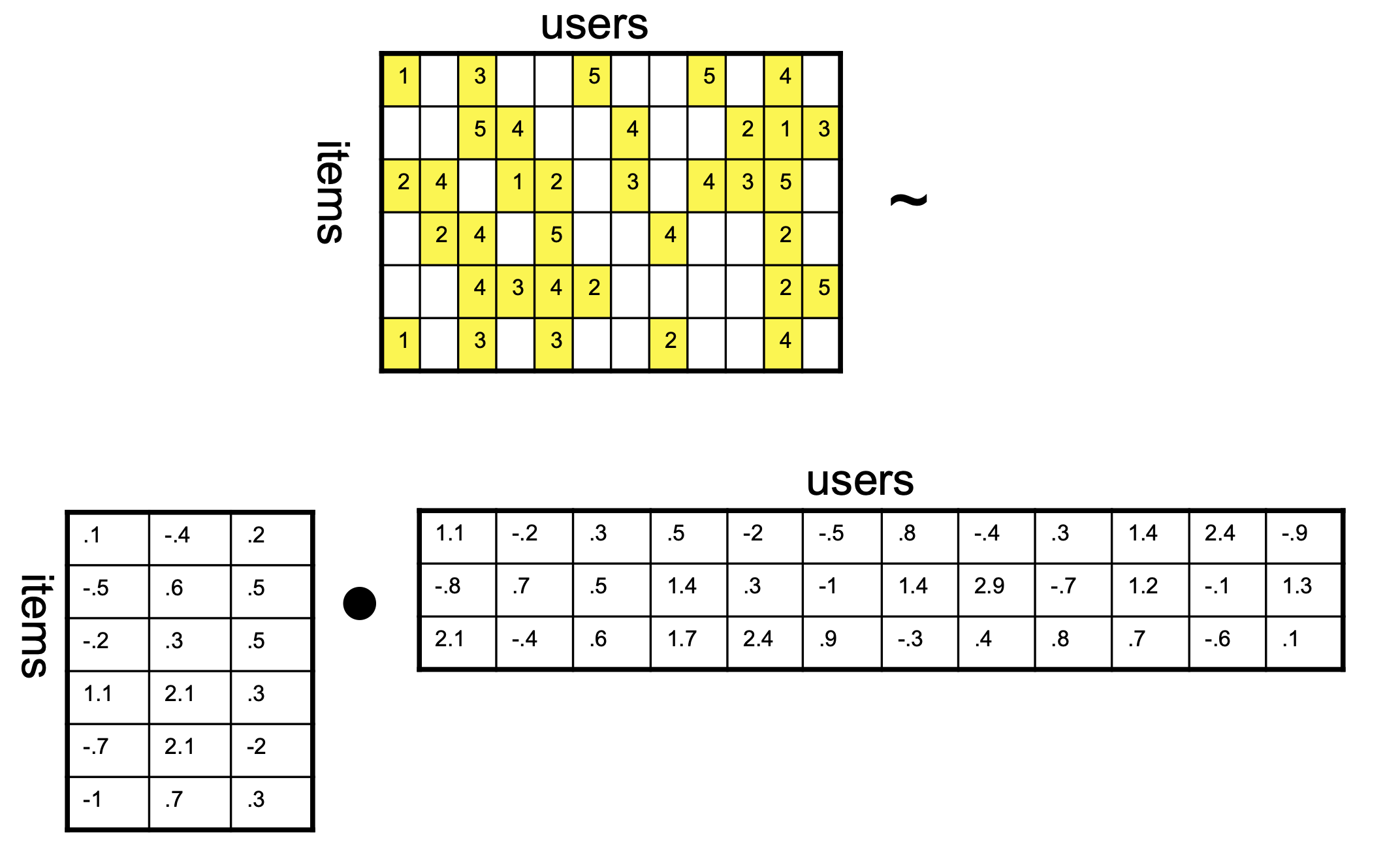
Nonetheless, we can imagine a situation like this:
where we decompose the ratings matrix \(R\) into two matrices. Each row of the left factor is an item vector \(\mathbf v_i\); each column of the right factor is a user vector \(\mathbf u_u\).
We want the product of the two matrices to be as close as possible to the known values of the ratings matrix.
What this setup implies is that our similarity function is the inner product.
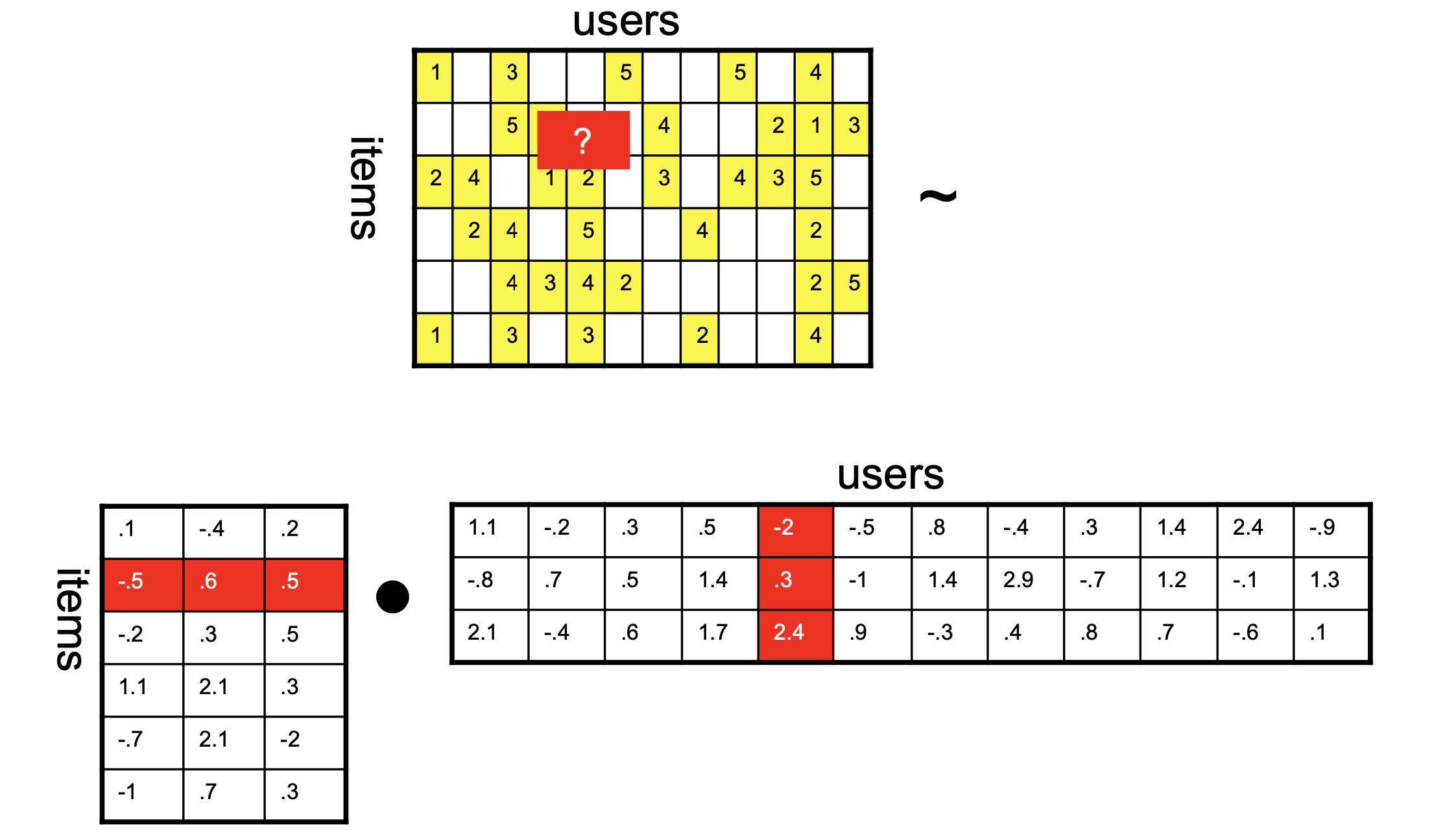
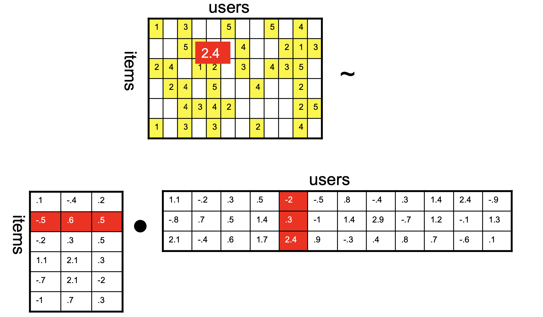
Which means that to predict an unknown rating, we take the inner product of latent vectors:
Taking, for example, item 2 (the 2nd row of the item factor) and user 5 (the 5th column of the user factor)…
This problem is not convex in \(U\) and \(V\) together, because of the product \(UV^T\). It is biconvex: convex in \(U\) when \(V\) is held fixed, and convex in \(V\) when \(U\) is held fixed.
In particular, if we hold either \(U\) or \(V\) constant, then the result is a simple ridge regression.
So one commonly used algorithm for this problem is called alternating least squares (ALS):
Hold \(U\) constant, and solve for \(V\)
Hold \(V\) constant, and solve for \(U\)
If not converged, go to Step 1.
The ALS Update
Hold \(V\) fixed. The objective splits into one small problem per user. For user \(u\), let \(J_u\) be the items she rated, \(V_{J_u}\) their rows of \(V\), and \(\mathbf r_{u,J_u}\) her ratings:
This is the ridge formula \(\hat{\boldsymbol\beta} = (X^TX + cI)^{-1}X^T\mathbf y\) with \(X = V_{J_u}\) (the item vectors are the features), \(\mathbf y = \mathbf r_{u,J_u}\) (her ratings) and \(c = \lambda\).
The other half-step is the mirror image: for item \(i\), regress the ratings it received on the factors of the users who rated it.
solve_U in scripts/recommender_als.py is exactly this line, once per user: np.linalg.solve(V[W[i]].T.dot(V[W[i]]) + I, V[W[i]].T.dot(x_i[W[i]])).
ALS Update: a Rank-1 Example
Take \(k = 1\), so every factor is a number. Fixed item factors: \(v_1 = 1\), \(v_2 = 2\), \(v_3 = 1.75\).
User \(u\) rated \(r_{u1} = 2\) and \(r_{u2} = 5\), and has not rated item 3.
The penalty pulls the factor toward 0, and every prediction shrinks with it: shrinkage. It costs some fit on the two ratings she gave, and protects against trusting a factor estimated from very few ratings.
The same numbers through the ridge formula:
Code
V_rated = np.array([[1.0], [2.0]]) # item factors of the items she ratedr_u = np.array([2.0, 5.0]) # her ratingsfor lam in [0, 1]: u_u = np.linalg.solve(V_rated.T @ V_rated + lam * np.eye(1), V_rated.T @ r_u)print(f'lambda = {lam}: u_u = {u_u[0]:.2f}, prediction for item 3 = {1.75* u_u[0]:.2f}')
The entire Amazon reviews dataset is too large to work with easily, and it is too sparse.
Hence, we will take the densest rows and columns of the matrix: users who wrote more than 50 reviews and movies with more than 50 reviews. Those star ratings are the file dense-block.csv.
Now we create a \(\textnormal{UserID} \times \textnormal{ProductID}\) matrix from these reviews.
Missing entries will be filled with NaNs.
Code
R = dense.pivot(index='UserId', columns='ProductId', values='Score')print(f"Review matrix shape: {R.shape}")print(f"Fraction of entries known: {R.count().sum() / R.size:.2%}")
Review matrix shape: (3677, 7244)
Fraction of entries known: 0.99%
Even this “dense” block is about 99% empty. A typical \(5 \times 4\) corner is all missing:
Code
R.iloc[900:905, 1000:1004]
ProductId
1417024917
1417030321
1417030976
1417054069
UserId
A1WLZYEOIL1HLT
NaN
NaN
NaN
NaN
A1WNJVA59HLMO5
NaN
NaN
NaN
NaN
A1WR12AC35R3K6
NaN
NaN
NaN
NaN
A1WSFHRBY2ZD1R
NaN
NaN
NaN
NaN
A1WUMTJOASEL5F
NaN
NaN
NaN
NaN
We’ll use code from the Antidote Data Framework to do the matrix factorization and ALS. We have local copies recommender_MF.py, recommender_als.py and recommender_lmafit.py in the scripts/ folder of our repository.
To evaluate honestly, we first hide 10% of the known ratings (per user), fit on the rest, and score the hidden ones.
import recommender_MF as MFnp.random.seed(0)omega_train, omega_val = MF.train_val_split(~R.isnull(), 0.1)R_train = R.where(omega_train)print(f'{omega_train.sum().sum():,} training ratings, {omega_val.sum().sum():,} held-out ratings')
236,710 training ratings, 26,332 held-out ratings
Fit rank 20 with \(\lambda = 1\) on the training ratings:
Rank 20 with \(\lambda = 1\) nearly memorises the training ratings — and does worse than the global mean on ratings it has not seen.
Fewer factors and a larger penalty give up training fit and win on held-out data.
\(k\) and \(\lambda\) are hyperparameters: tune them on a validation split, report a test split.
What Held-Out RMSE Cannot Tell You
Ratings are missing not at random. People rate what they chose to watch, and mostly what they liked. Held-out RMSE is measured on that same biased sample, so it flatters popular items and says little about the rest of the catalogue.
A recommender ships a list, not a number. What the product needs is a good top-\(k\) list per user, measured by precision@\(k\) or recall@\(k\). A model can win on RMSE and lose on ranking.
Offline ≠ online. Whether recommendations change what people watch or buy is measured with an A/B test on live traffic.
Assessing Matrix Factorization
Matrix Factorization per se is a good idea.
However, many of the improvements we’ve discussed for CF apply to MF as well.
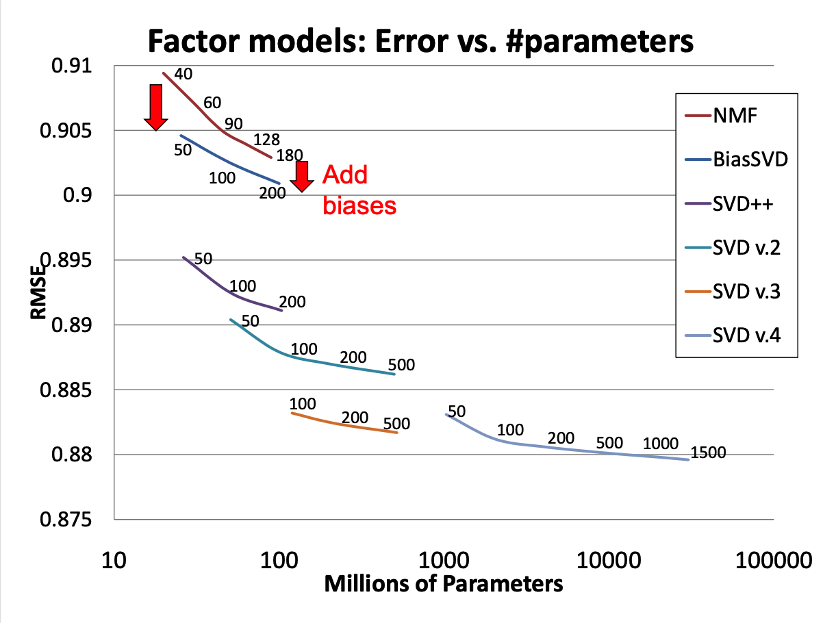
To illustrate, we’ll look at some of the successive improvements used by the team that won the Netflix prize (“BellKor’s Pragmatic Chaos”).
When the prize was announced, the Netflix supplied solution achieved an RMSE of 0.951.
By the end of the competition (about 3 years), the winning team’s solution achieved RMSE of 0.856.
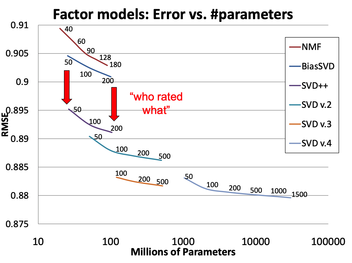
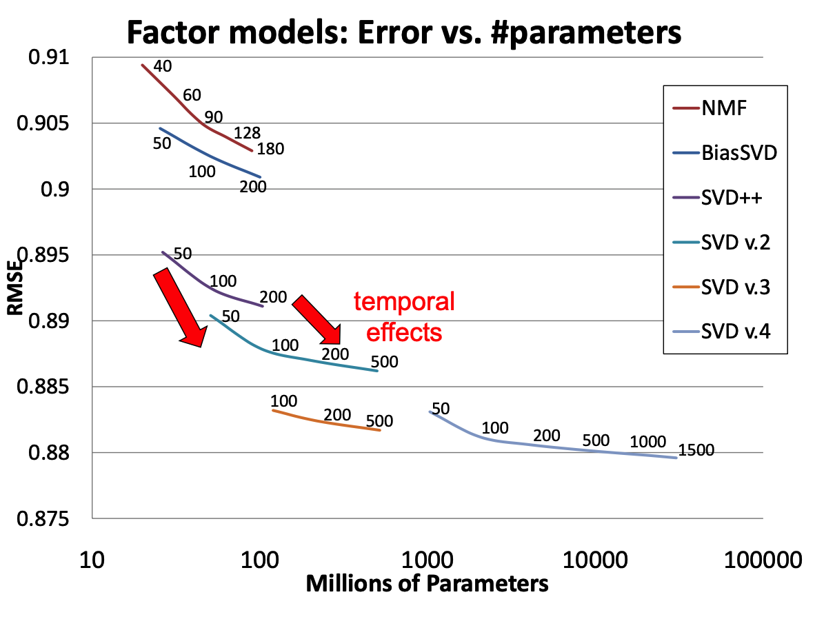
Figure 2: Matrix factorization models’ accuracy. The plots show the root-mean-square error of each of four individual factor models (lower is better). Accuracy improves when the factor model’s dimensionality (denoted by numbers on the charts) increases. In addition, the more refined factor models, whose descriptions involve more distinct sets of parameters, are more accurate.
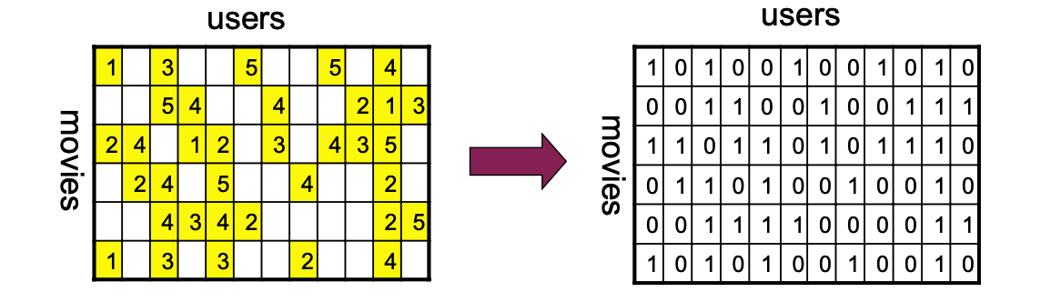
2. Who Rated What?
In reality, ratings are not provided at random.
Take note of which users rated the same movies (ala CF) and use this information.
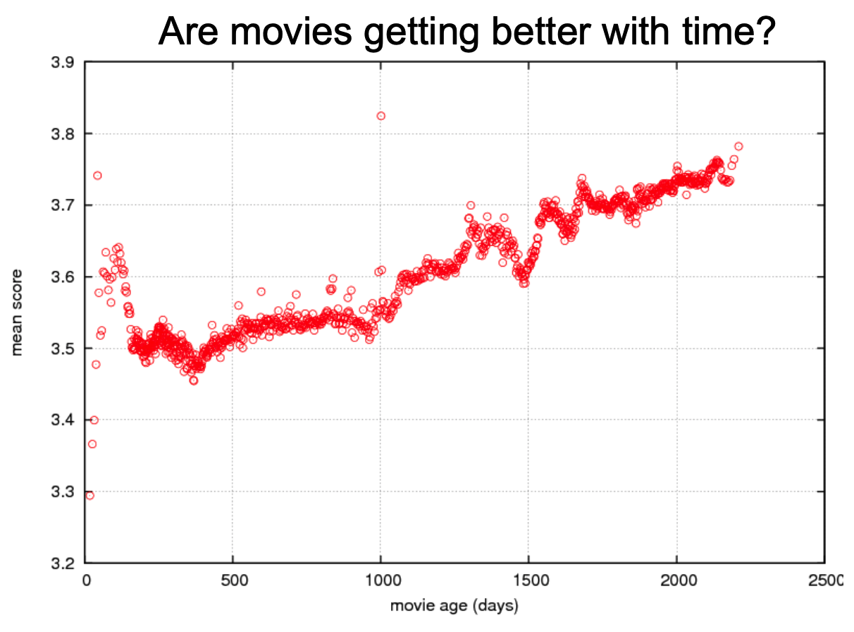
3. Ratings Change Over Time
Older movies tend to get higher ratings!
If we add time-varying biases, and let each user’s taste drift (the item factors stay fixed) (Koren 2009):
With the time and implicit-feedback terms the model is no longer bilinear in two blocks of parameters, so the Netflix teams fit it with stochastic gradient descent (Lecture 16) rather than ALS.
Cold Start
Everything so far needs a history. A new user signs up and has rated nothing.
CF: user–user has no co-rated items, so no similarities; item–item has no items she rated, so the neighbourhood \(n_k(i, u)\) is empty.
MF: no term \((r_{ui} - \mathbf u_u^T\mathbf v_i)^2\) involves her, so only \(\lambda\Vert\mathbf u_{\text{new}}\Vert^2\) does. It is minimised at \(\mathbf u_{\text{new}} = \mathbf 0\) (the ALS formula with \(J_u\) empty), so \(\hat r = 0\) for every item. With \(\lambda = 0\) her factor is undetermined.
MF with biases:\(\alpha_{\text{new}} = 0\) too, so \(\hat r_{ui} = \mu + \beta_i\): the same popular-items list for everyone. Better, but not personal.
New item: the mirror image. \(\mathbf v_{\text{new}} = \mathbf 0\), so it scores 0 for everyone and is never recommended.
Mitigations — every real system is a hybrid:
Onboarding: ask for a few ratings at sign-up (“pick three titles you like”).
Content and metadata: genre, cast, description text, or user demographics place a new item or user in the latent space before any ratings exist.
Popularity prior: recommend what is popular (or \(\mu + \beta_i\)) at first.
Blend: weight the prior heavily at first and shift to the collaborative prediction as ratings arrive.
Recap
Recommender systems predict a sparse, skewed user–item ratings matrix; the global mean is the baseline to beat.
Collaborative filtering: item–item or user–user \(k\)-NN with correlation over co-raters, after removing biases; compare along the short side.
Matrix factorization: users and items in one latent space, \(\hat r_{ui} = \mathbf u_u^T\mathbf v_i\), fitted on observed entries only by ALS — one ridge regression per row.
Evaluate on held-out ratings: training RMSE flatters, and RMSE itself is not the product metric.
Cold start: with no history, CF and MF fall back to the mean or popularity; hybrids fill the gap.
References
Koren, Yehuda. 2009. “Collaborative Filtering with Temporal Dynamics.”Proceedings of the 15th ACM SIGKDD International Conference on Knowledge Discovery and Data Mining 42: 447–56. https://dl.acm.org/doi/10.1145/1557019.1557072.
Koren, Yehuda, Robert Bell, and Chris Volinsky. 2009. “Matrix Factorization Techniques for Recommender Systems.”Computer 42 (8): 30–37. https://ieeexplore.ieee.org/document/5197422.
Linden, Greg, Brent Smith, and Jeremy York. 2003. “Amazon.com Recommendations: Item-to-Item Collaborative Filtering.”IEEE Internet Computing 7 (1): 76–80. https://doi.org/10.1109/MIC.2003.1167344.
Naumov, Maxim et al. 2019. “Deep Learning Recommendation Model for Personalization and Recommendation Systems.”arXiv Preprint arXiv:1906.00091, May. http://arxiv.org/abs/1906.00091.
Sarwar, Badrul, George Karypis, Joseph Konstan, and John Riedl. 2001. “Item-Based Collaborative Filtering Recommendation Algorithms.”Proceedings of the 10th International Conference on World Wide Web, 285–95. https://doi.org/10.1145/371920.372071.