Recap: Introduction to Networks
DS701 Session 23 — Mon Nov 23, 2026
A graph is nodes + edges — and the adjacency matrix is the graph
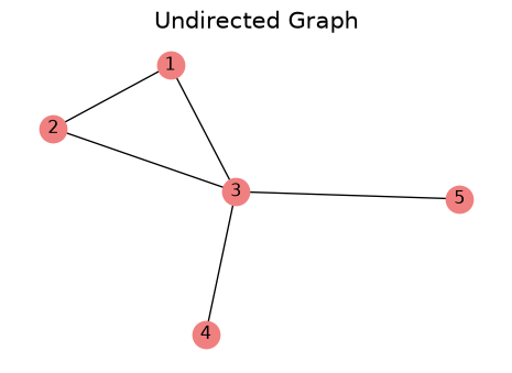
\(E = \{(1,2),(1,3),(2,3),(3,4),(3,5)\}\)
Number the nodes; \(A_{ij} = 1\) if \((i,j) \in E\), else \(0\):
\[ A = \begin{bmatrix} 0 & 1 & 1 & 0 & 0\\ 1 & 0 & 1 & 0 & 0\\ 1 & 1 & 0 & 1 & 1\\ 0 & 0 & 1 & 0 & 0\\ 0 & 0 & 1 & 0 & 0 \end{bmatrix} \qquad \text{row sums} = \begin{bmatrix} 2\\2\\4\\1\\1 \end{bmatrix} \]
- Edge list and \(A\) carry the same information — nothing is lost either way.
- Degree = row sum. Total \(= 10 = 2e\).
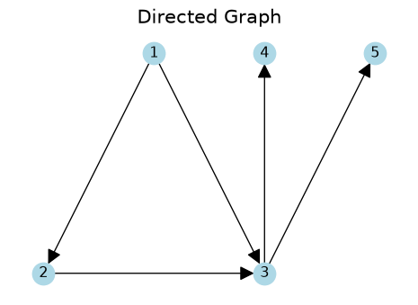
- Undirected \(\Leftrightarrow\) \(A\) symmetric. Directed: row \(i\) = out-edges, column \(j\) = in-edges — node 1 has in-degree 0, out-degree 2; node 3 has 2 and 2.
- Directed paths run head-to-tail: 1 → 3 → 5 exists, 5 → 1 does not. Reachability becomes one-way.
- Weighted: put the weight where the 1 was.
Real networks I: heavy tails
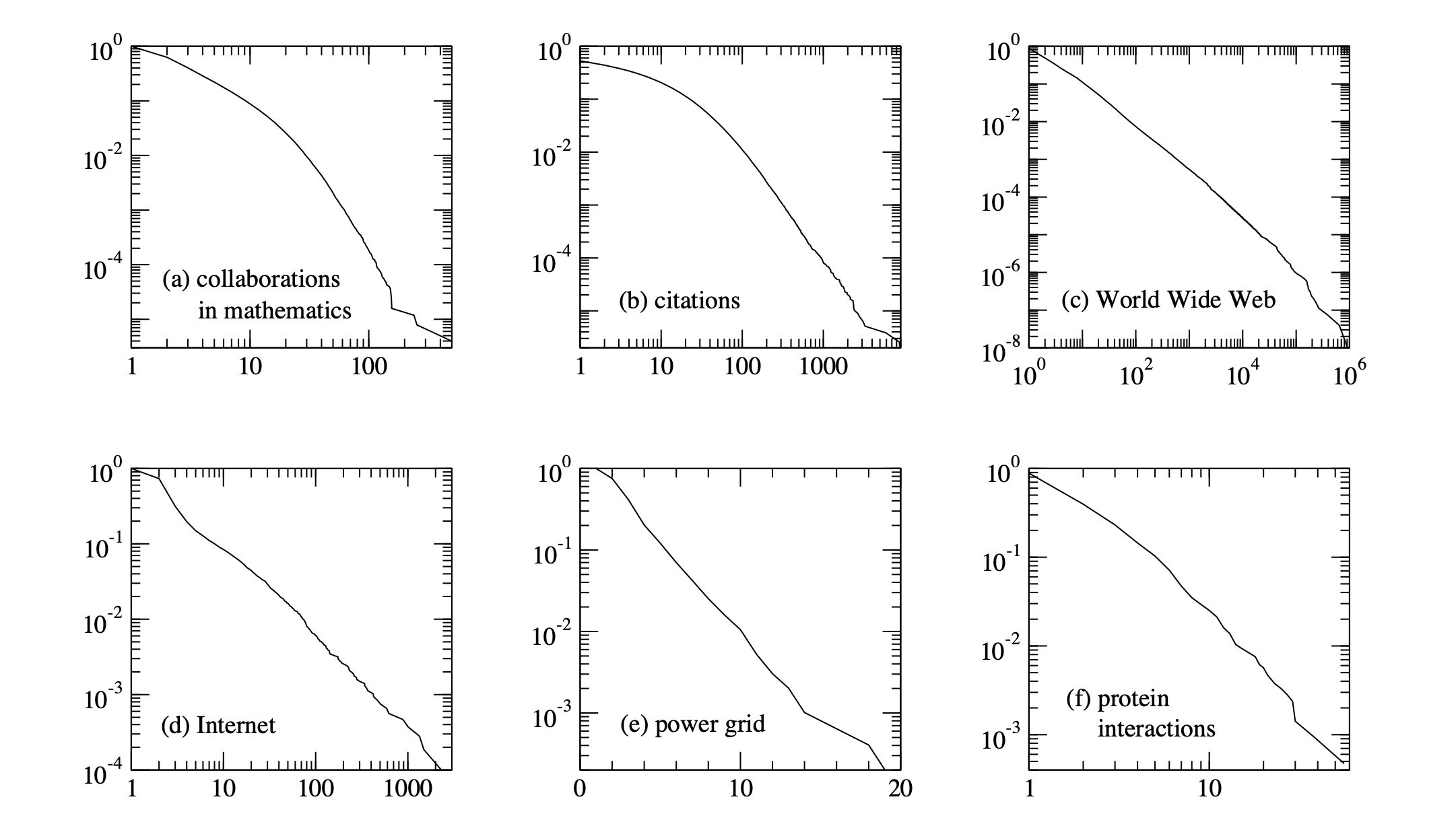
Degree distribution as a CCDF: \(P(X > x)\), the fraction of nodes with degree above \(x\).
- Power law / Pareto: \(P(X > x) = (k/x)^{\alpha}\) — a straight line on log–log axes, slope \(-\alpha\).
- Meaning: most nodes have few neighbours; a small but real set of nodes have very many. Hubs.
- \(G(n,p)\) with the same mean would show no such tail — its log–log plot falls off a cliff.
- Not universal: the power grid (e) is straight on lin–log axes — an exponential tail.
Real networks II: clustering, and the small world
Clustering coefficient — the probability that two of your neighbours are connected.
\[ C^{(1)} = \frac{\sum_i \#\text{triangles at } i}{\sum_i \#\text{neighbour pairs at } i} \]
Five-node example: \(\dfrac{1+1+1}{1+1+6} = \dfrac{3}{8}\).
\(C^{(2)}\) averages the per-node ratios instead (nx.average_clustering): \(\dfrac{1}{5}\bigl(1+1+\tfrac16\bigr) = 0.433\).
Random graph: \(C = p\). Real networks: much higher.
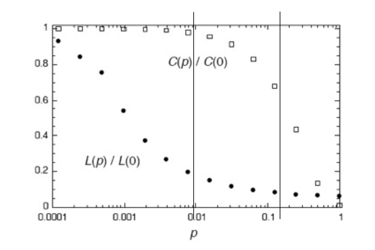
Watts–Strogatz: a few rewired edges collapse \(L\) while \(C\) holds. Small world = high clustering and short paths. Milgram’s 6.2 hops; Granovetter’s weak ties; Kevin Bacon is not special.
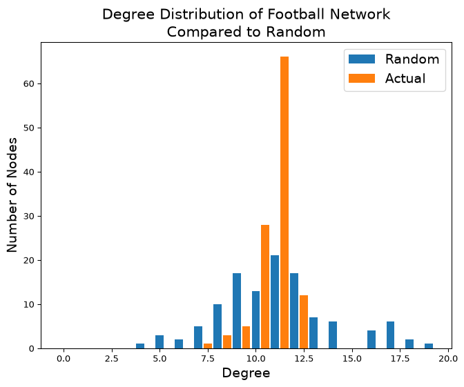
Putting it together: football vs. random
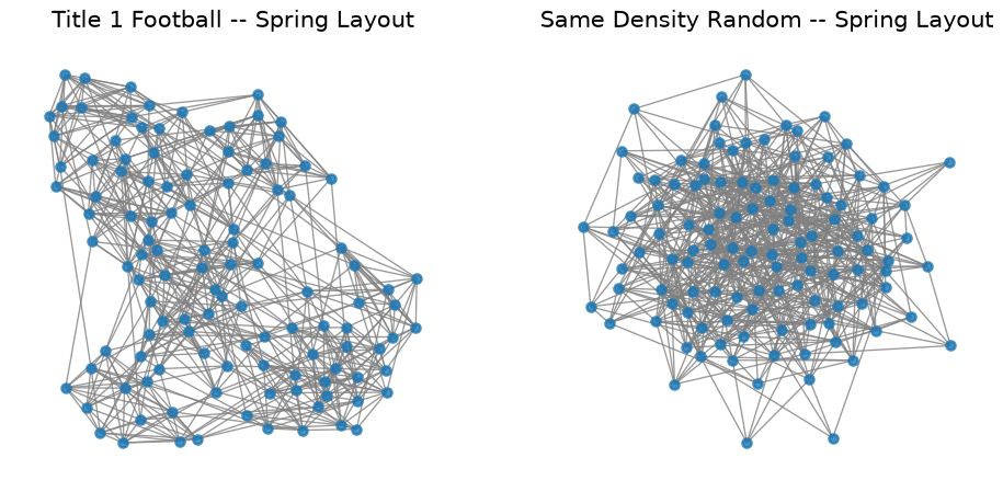
- Same \(n\), same \(e\). Spring layout: conferences clump; the random graph is a blob.
- Clustering coefficient: real \(\gg\) random. Diameter and average path: both short.
- Degree histogram: a spike at 11 games — a scheduling rule. “Different from random” here means more regular, not heavier-tailed. The baseline tells you that there is structure; you still have to say what.
Activity: build the graph, then change what “the graph” means
Goal: build small networks in NetworkX from edge lists — adjacency matrix, degree, components, shortest paths, diameter, clustering, degree distributions against a \(G(n,p)\) baseline and a heavy-tailed one — then re-represent the same data as directed / weighted / thresholded graphs and watch the answers move.
- Work in groups of 2–3. Open your section’s notebook.
- Parts marked (autograded) are submitted to Gradescope; the rest is participation.
- Staff will circulate — be ready to explain any part of your work.
- Dependencies:
numpy,pandas,matplotlib,scipy,networkx.
Section A1 

Section B1
The activity notebook goes live on the day of the lecture. Colab is optional — you can also open it on GitHub and run it locally.