We know that a model that overfits does not generalize well. In other words, the model does not perform well on data it was not trained on.
We observe overfitting when the training accuracy of the model is high, while the accuracy on the validation set (or held out test set) stagnates.
In this lecture we will discuss regularization. A technique to help prevent overfitting. We will see how to apply regularization to regression problems.
However, regularization is a general technique to ensure models learn broad patterns and is applicable in neural networks.
What is regularization?
We know regularization is a way to prevent overfitting, but how does this actually work?
The idea behind regularization is to penalize a model’s loss function during training. The added penalty will discourage the model from becoming too complex (i.e., overfitting).
In regression, our training process was to compute coefficients \(\boldsymbol{\beta}\) by minimizing
\[
\min_{\boldsymbol{\beta}} \Vert X \boldsymbol{\beta} - \mathbf{y}\Vert_{2}^{2},
\]
where, as in the linear regression lecture, \(X\in\mathbb{R}^{n\times p}\) is the design matrix with one row per observation (\(n\) observations, \(p\) features) and \(\mathbf{y}\in\mathbb{R}^{n}\) holds the dependent variable.
What is regularization?
Regularization adds a function \(R(\boldsymbol{\beta})\) to the minimization problem. A regularized minimization problem is then: compute \(\boldsymbol{\beta}\) such that
\[
\min_{\boldsymbol{\beta}} \Vert X \boldsymbol{\beta} - \mathbf{y}\Vert_{2}^{2} + cR(\boldsymbol{\beta}).
\]
The regularization coefficient \(c\) is a hyperparameter that controls the importance of the regularization term \(R(\boldsymbol{\beta})\).
We will consider two common forms of \(R(\boldsymbol{\beta})\):
\(R(\boldsymbol{\beta}) = \Vert \boldsymbol{\beta}\Vert_{2}^{2}\), called ridge regression, and
\(R(\boldsymbol{\beta}) = \Vert \boldsymbol{\beta}\Vert_1\), called LASSO regression.
Multicollinearity
In statistics, multicollinearity (also collinearity) is a phenomenon in which two or more predictor variables in a multiple regression model are highly correlated, meaning that one can be linearly predicted from the others with a substantial degree of accuracy.
We will see that multicollinearity can be problematic in our regression models.
To address these issues, we will consider
What are the potential sources for multicollinearity?
What does multicollinearity tell us about our data?
Understanding these questions will inform us how regularization can be used to mitigate the issue of multicollinearity.
Sources of Multicollinearity
We will be working with our design matrix \(X\in\mathbb{R}^{n\times p}\), where each row corresponds to an observation and the \(p\) columns are the \(p\) features.
We will see that multicollinearity arises when the columns of \(X\) are linearly dependent (or nearly linearly dependent).
As a consequence, the matrix \(X^{T}X\) is no longer invertible. However, as we saw in our Linear Regression lecture, the least squares solution still exists. It is just not unique.
Sources of Multicollinearity
What are the situations where this can happen?
One clear case is when \(n < p\), which means \(X\) has more columns than rows. That is, there are more features than there are observations in the data.
However, we can still observe multicollinearity when \(n > p\).
This can happen when the columns of \(X\) happen to be linearly dependent because of the nature of the data itself. In particular, this happens when one column is a linear function of the other columns. This means that one independent variable is a linear function of one or more of the others.
Unfortunately, in practice we will run into trouble even if variables are almost linearly dependent.
The Longley Dataset
To illustrate the multicollinearity problem, we’ll load a standard dataset.
The Longley dataset contains various US macroeconomic variables from 1947–1962.
We have the following features:
GNP - GNP (Gross National Product)
GNPDEFL - GNP deflator, a way to account for inflation over different years
                            OLS Regression Results
==============================================================================
Dep. Variable:                 TOTEMP   R-squared:                       0.987
Model:                            OLS   Adj. R-squared:                  0.981
Method:                 Least Squares   F-statistic:                     156.4
Date:                Sat, 17 Oct 2026   Prob (F-statistic):           3.70e-09
Time:                        20:04:10   Log-Likelihood:                -117.83
No. Observations:                  16   AIC:                             247.7
Df Residuals:                      10   BIC:                             252.3
Df Model:                           5
Covariance Type:            nonrobust
==============================================================================
                 coef    std err          t      P>|t|      [0.025      0.975]
------------------------------------------------------------------------------
GNPDEFL      -48.4628    132.248     -0.366      0.722    -343.129     246.204
GNP            0.0720      0.032      2.269      0.047       0.001       0.143
UNEMP         -0.4039      0.439     -0.921      0.379      -1.381       0.573
ARMED         -0.5605      0.284     -1.975      0.077      -1.193       0.072
POP           -0.4035      0.330     -1.222      0.250      -1.139       0.332
const       9.246e+04   3.52e+04      2.629      0.025    1.41e+04    1.71e+05
==============================================================================
Omnibus:                        1.572   Durbin-Watson:                   1.248
Prob(Omnibus):                  0.456   Jarque-Bera (JB):                0.642
Skew:                           0.489   Prob(JB):                        0.725
Kurtosis:                       3.079   Cond. No.                     1.21e+08
==============================================================================

Notes:
[1] Standard Errors assume that the covariance matrix of the errors is correctly specified.
[2] The condition number is large, 1.21e+08. This might indicate that there are
strong multicollinearity or other numerical problems.
Condition Number
The notion of conditioning pertains to the perturbation behavior of a mathematical problem. A well-conditioned problem is one where small changes to the inputs produce small changes to the output. An ill-conditioned problem is one where small changes in the input can produce very large changes in the output.
The condition number of a matrix provides an indication of how accurately you can compute with it.
A large condition number tells us that our problem is ill conditioned, i.e., small changes to the input can produce very large changes in the output.
A small condition number tells us that our problem is well-conditioned.
Condition Number
The condition number is derived using matrix norms, which is beyond the scope of this course. However, we will use the following definition for the condition number of our matrix
This means that if we have a poorly conditioned data matrix \(X\), then \(X^TX\) is even more poorly conditioned.
This is why, in practice, you should not form\(X^TX\) and invert it. The normal equations describe the solution; good solvers (np.linalg.lstsq, sm.OLS) reach the same \(\hat{\boldsymbol{\beta}}\) by working with \(X\) directly, at condition number \(\kappa(X)\) rather than \(\kappa(X)^2\).
Normal Equations: a callback
From the linear regression lecture: the least-squares solution satisfies the normal equations \(X^TX\boldsymbol{\beta} = X^T\mathbf{y}\), which always have at least one solution.
The solution is unique exactly when \(X^TX\) is invertible, i.e. when the columns of \(X\) are linearly independent.
If the columns are linearly dependent, \(X^TX\) has a zero singular value, \(\kappa(X^TX) = \infty\), and \((X^TX)^{-1}\) does not exist. There are then infinitely many \(\boldsymbol{\beta}\) with the same fitted values \(X\boldsymbol{\beta}\) and the same residual norm: the fit is determined, the coefficients are not.
This is the simplest kind of multicollinearity. It is a problem of interpretation, not of prediction.
Near Linear Dependence
Near linear dependence causes problems as well. This can happen, for example, due to measurement errors. Or when two or more columns are strongly correlated.
In such a situation, we have some column of our design matrix that is close to being a linear combination of the other columns.
When these situations occur we will have problems with linear regression.
Near Linear Dependence
As a result of near linear dependence, the smallest singular value of the design matrix \(X\) will be close to zero. This means that \(\kappa(X)\) will be very large.
The condition number tells us that a small change in the input to our problem can result in large changes to the output.
This means that for a design matrix \(X\) with near linearly dependent columns, the values we compute for \(\boldsymbol{\beta}\) in our linear regression can vary significantly.
Put in the language of Generalization: an unstable \(\hat{\boldsymbol{\beta}}\)isvariance. Refit on a slightly different sample and the coefficients swing, so each individual fit has chased noise. The cure for variance there was to constrain the model; here the constraint is a penalty on \(\boldsymbol{\beta}\), which regularizes the solution.
Longley: reading the condition number
Recall that the condition number of our data is around \(10^8\).
A large condition number is evidence of a problem.
As a general rule of thumb:
If the condition number is less than 100, there is no serious problem with multicollinearity.
Condition numbers between 100 and 1000 imply moderate to strong multicollinearity.
Condition numbers bigger than 1000 indicate severe multicollinearity.
Longley: which columns are nearly dependent?
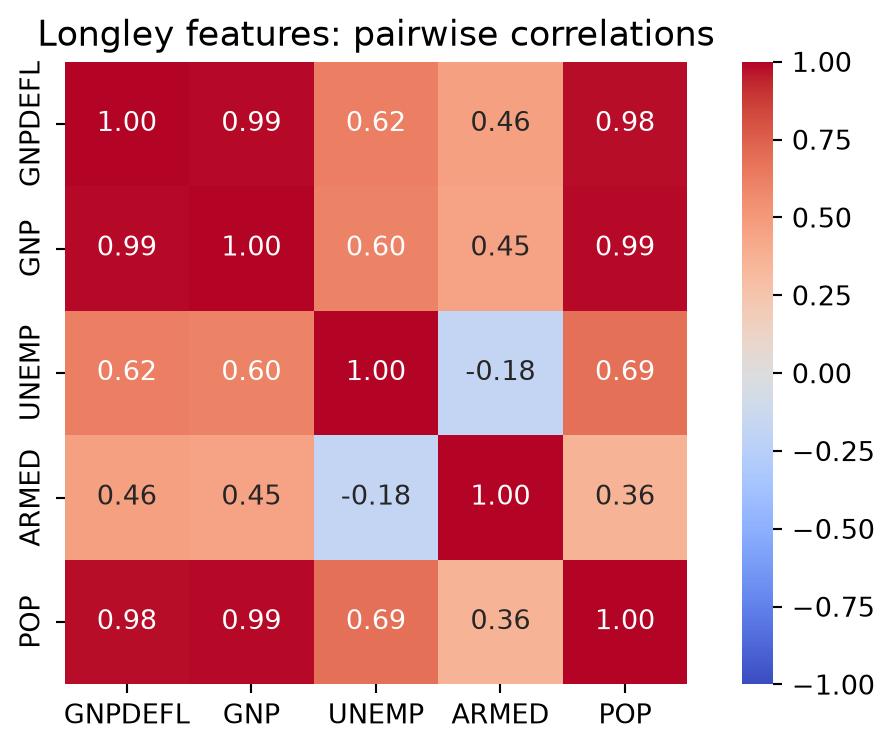
The correlation matrix of the features shows where the near-dependence comes from.
We can see very strong linear relationships between GNP Deflator, GNP, and Population (correlations above 0.97): three columns carrying essentially one piece of information.
Addressing Multicollinearity
Here are two strategies we can employ to address multicollinearity:
Ridge Regression
Model Selection via LASSO
Why the coefficients blow up
The first thing to note is that when columns of \(X\) are nearly dependent, the components of \(\hat{\boldsymbol{\beta}}\) tend to be large in magnitude.
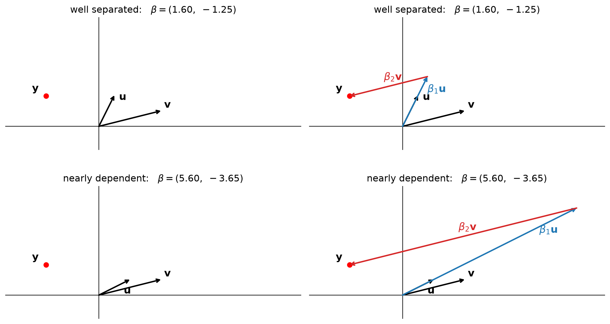
Consider a regression in which we are predicting the point \(\mathbf{y}\) as a linear combination \(\beta_1\mathbf{u} + \beta_2\mathbf{v}\) of two \(X\) columns \(\mathbf{u}\) and \(\mathbf{v}\). In two dimensions this is exact, and the coefficients are the solution of a \(2\times 2\) system, computed below with np.linalg.solve.
Top row:\(\mathbf{u}\) and \(\mathbf{v}\) point in clearly different directions, and the same \(\mathbf{y}\) is reached with coefficients of modest size, \(\boldsymbol{\beta} = (1.60, -1.25)\).
Bottom row:\(\mathbf{u}\) and \(\mathbf{v}\) are nearly parallel. The part of \(\mathbf{y}\) that points away from their shared direction can only be built as the difference of two long, nearly cancelling vectors: \(\boldsymbol{\beta} = (5.60, -3.65)\), more than three times as large for the same target.
Push \(\mathbf{u}\) and \(\mathbf{v}\) closer still and the coefficients grow without bound – and flip wildly if \(\mathbf{y}\) moves a little.
This geometric argument illustrates why the regression coefficients will be very large under multicollinearity. As a result, \(\Vert\boldsymbol{\beta}\Vert_2\) will be very large – which is exactly what ridge regression penalizes.
Ridge Regression
Ridge regression adjusts the least squares regression by shrinking the estimated coefficients towards zero.
The purpose is to fix the magnitude inflation of \(\Vert\boldsymbol{\beta}\Vert_2\).
To do this, Ridge regression assumes that the model has no intercept term – both the response and the predictors have been centered so that \(\beta_0 = 0\).
Ridge regression then consists of adding a penalty term to the regression:
For any given \(c\) this has a closed-form solution in which \(\hat{\boldsymbol{\beta}} = (X^TX +cI)^{−1}X^T\mathbf{y}.\)
The solution to the Ridge regression problem always exists and is unique, even when the data contains multicollinearity: adding \(c\) to every eigenvalue of \(X^TX\) lifts the smallest one off zero.
Here, \(c \geq 0\) is a tradeoff parameter and controls the strength of the penalty term:
When \(c = 0\), we get the least squares estimator: \(\hat{\boldsymbol{\beta}} = (X^TX)^{−1}X^T\mathbf{y}\)
When \(c \rightarrow \infty\), we get \(\hat{\boldsymbol{\beta}} \rightarrow 0.\)
Increasing the value of \(c\) forces the norm of \(\hat{\boldsymbol{\beta}}\) to decrease, yielding smaller coefficient estimates in magnitude.
For a finite, positive value of \(c\), we are balancing two tasks: fitting a linear model and shrinking the coefficients.
The coefficient \(c\) is a hyperparameter that controls the model complexity. We typically set \(c\) by holding out data, i.e., cross-validation.
Ridge in one dimension
With a single centered (mean-subtracted) column \(\mathbf{x}\), write the sum of squares as \(s = \mathbf{x}^T\mathbf{x}\).
Then \(\hat\beta_{LS} = \mathbf{x}^T\mathbf{y}/s\) is the least-squares slope/solution.
Expanding the squared error around it, \(\Vert\mathbf{y} - \mathbf{x}\beta\Vert_2^2 = s\,(\beta - \hat\beta_{LS})^2 + \text{const}\), so ridge minimizes
Ridge multiplies the least-squares estimate by a factor in \((0, 1)\): it shrinks, but never reaches zero for finite \(c\).
For a standardized column \(s = \mathbf{x}^T\mathbf{x} = n\), so the shrinkage factor is \(1/(1 + c/n)\): a penalty of \(c = n\) halves every coefficient. (Keep this in mind when reading the \(c\) axis of the plots below – \(c\) is on the scale of \(n\).)
In many dimensions the same thing happens along each singular direction of \(X\), with factor \(\sigma_j^2/(\sigma_j^2 + c)\): the directions with tiny \(\sigma_j\) – the nearly dependent ones – are shrunk the most. That is the next lecture’s story.
Scaling
Note that the penalty term \(\Vert\boldsymbol{\beta}\Vert_2^2\) would be unfair to the different predictors if they are not on the same scale: a useful feature measured in tiny units needs a huge coefficient and is punished for it, while a feature in huge units is nearly free.
Therefore, if we know that the variables are not measured in the same units, we first standardize the columns of \(X\) (zero mean, unit variance) and center \(\mathbf{y}\), and then perform ridge regression.
By centering \(\mathbf{y}\) and \(X\) we do not need (or include) an intercept in the model – and the intercept should never be penalized.
Fit the scaler on the training split only. The means and standard deviations are part of the model; computing them on data you will later test on leaks test information into training.
Another name for ridge regression is Tikhonov regularization. You may see this terminology used in textbooks on optimization.
Ames housing: a data set for the sweeps
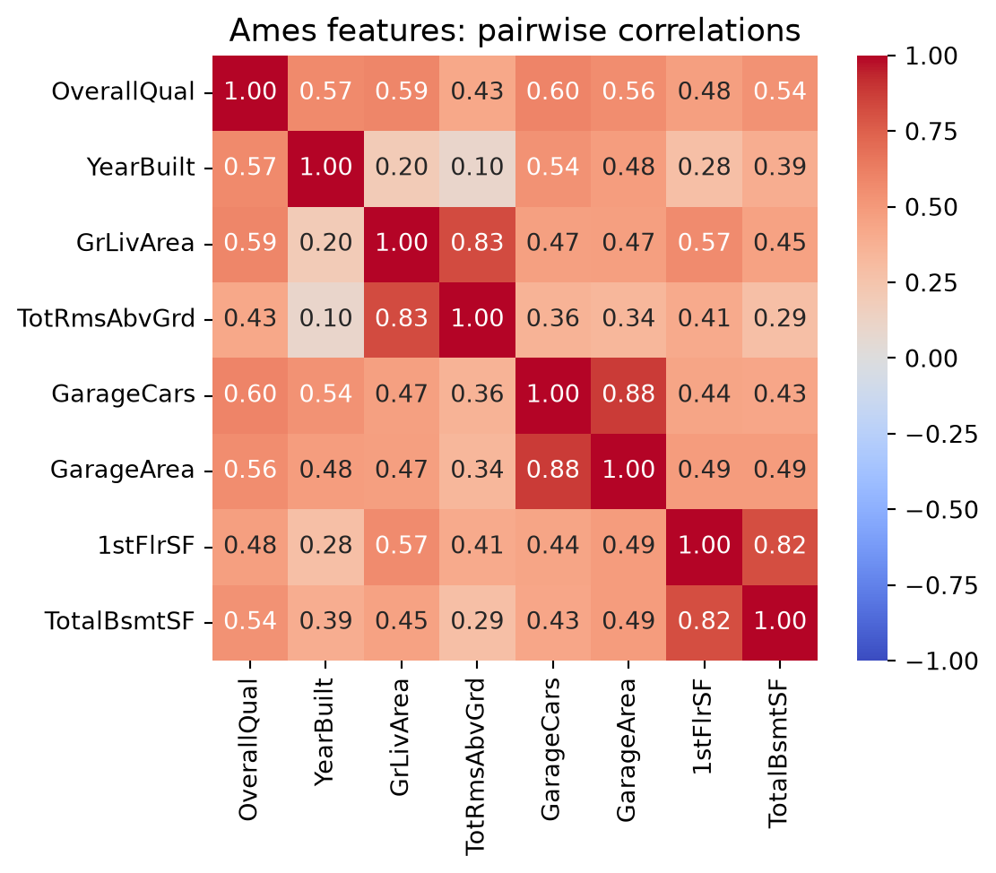
Longley has only 16 rows – fine for showing a condition number, hopeless for cross-validation (8 training points for 5 features). For the penalty sweeps we switch to the Ames housing data from the linear regression lecture: 1460 houses, target SalePrice, and eight numeric features chosen to include three genuinely collinear pairs.
Code
import os, urllib.requestdef data_file(path):"""Course data file: use a local copy (here, or in the repo root above a notebook in jupyter_notebooks/), else fetch it from the Materials repo (Colab)."""for prefix in ('', '../'):if os.path.exists(prefix + path):return prefix + path os.makedirs(os.path.dirname(path) or'.', exist_ok=True) urllib.request.urlretrieve('https://raw.githubusercontent.com/tools4ds/DS701-Materials-FA26/main/'+ path, path)return pathames = pd.read_csv(data_file('data/ames-housing-data/train.csv'))ames_features = ['OverallQual', 'YearBuilt','GrLivArea', 'TotRmsAbvGrd', # living area vs number of rooms'GarageCars', 'GarageArea', # garage capacity two ways'1stFlrSF', 'TotalBsmtSF'] # first floor sits on the basementX_ames = ames[ames_features]y_ames = ames['SalePrice']print(X_ames.shape)X_ames.describe().loc[['mean', 'std', 'min', 'max']].round(0)
The three pairs correlate at 0.83, 0.88 and 0.82. Nothing here is exactly dependent, so least squares runs – but, as the geometry predicted, it has to decide how to split one effect between two near-duplicate columns, and that decision is unstable.
Ridge on Ames: the held-out sweep
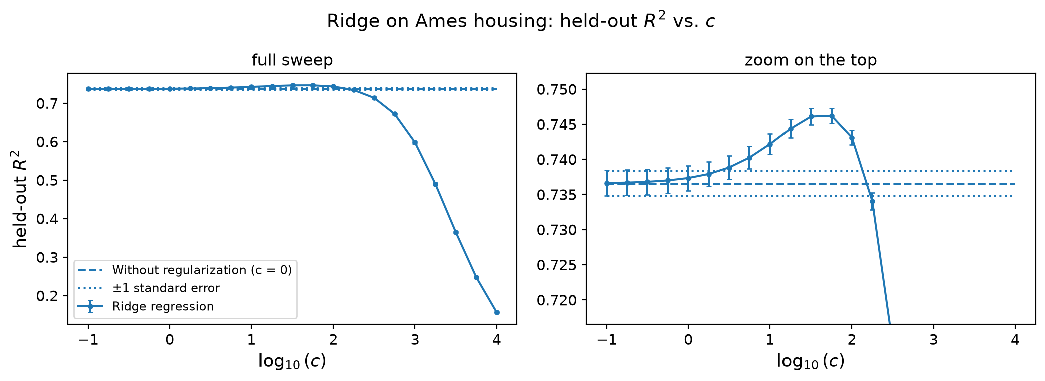
For each \(c\) we repeat 100 random train/test splits. To make the variance of \(\hat{\boldsymbol{\beta}}\) – the thing the penalty controls – visible, we train on a deliberately small 20% split (292 houses) and test on the other 80%. The scaler is fit on the training split each time. We use sklearn’s Ridge, whose alpha is exactly our \(c\).
Code
def heldout_sweep(make_model, c_values, X, y, nreps=100, test_size=0.8):"""Mean held-out R^2 (with standard error) and mean coefficients for each c.""" scores, coefs = [], []for c in c_values: r2s, betas = [], []for rep inrange(nreps): X_tr, X_te, y_tr, y_te = model_selection.train_test_split( X, y, test_size=test_size, random_state=rep) x_scaler = StandardScaler().fit(X_tr) # training split only y_scaler = StandardScaler().fit(y_tr.to_frame()) X_tr_s, X_te_s = x_scaler.transform(X_tr), x_scaler.transform(X_te) y_tr_s = y_scaler.transform(y_tr.to_frame()).ravel() y_te_s = y_scaler.transform(y_te.to_frame()).ravel() model = make_model(c, len(y_tr_s)).fit(X_tr_s, y_tr_s) r2s.append(r2_score(y_te_s, model.predict(X_te_s))) betas.append(model.coef_) scores.append([c, np.mean(r2s), np.std(r2s) / np.sqrt(nreps)]) coefs.append(np.mean(betas, axis=0))return np.array(scores), pd.DataFrame(coefs, index=c_values, columns=X.columns)def plot_sweep(scores, label, title):"""scores[0] is the unpenalized (c = 0) baseline; the rest are plotted vs log10(c). Left: the whole sweep. Right: zoomed in on the top, where the gain over c = 0 lives.""" base, sweep = scores[0], scores[1:] fig, axs = plt.subplots(1, 2, figsize=(11, 4)) span = [np.log10(sweep[0, 0]), np.log10(sweep[-1, 0])]for ax in axs: ax.errorbar(np.log10(sweep[:, 0]), sweep[:, 1], sweep[:, 2], marker='o', ms=3, capsize=2, label=label) ax.hlines(base[1], *span, linestyles='dashed', label='Without regularization (c = 0)') ax.hlines([base[1] - base[2], base[1] + base[2]], *span, linestyles='dotted', label=r'$\pm 1$ standard error') ax.set_xlabel(r'$\log_{10}(c)$', fontsize=13) ax.tick_params(labelsize=11) axs[0].set_ylabel('held-out $R^2$', fontsize=13) axs[0].set_title('full sweep', fontsize=12) axs[0].legend(loc='lower left', fontsize=9) axs[1].set_ylim(base[1] -0.02, sweep[:, 1].max() +0.006) axs[1].set_title('zoom on the top', fontsize=12) fig.suptitle(title, fontsize=14) plt.tight_layout()return axsdef ridge_model(c, n_train):return Ridge(alpha=c, fit_intercept=False) if c >0else LinearRegression(fit_intercept=False)ridge_cs = np.r_[0, 10** np.linspace(-1, 4, 21)]ridge_scores, ridge_coefs = heldout_sweep(ridge_model, ridge_cs, X_ames, y_ames)
Code
plot_sweep(ridge_scores, 'Ridge regression', 'Ridge on Ames housing: held-out $R^2$ vs. $c$')plt.show()
Reading the ridge sweep
For small \(c\) nothing changes: the penalty is negligible next to the squared error.
Around \(c \approx 10\)–\(100\) (recall \(n = 292\), so this is shrinkage of roughly 5–25%) the held-out \(R^2\) rises above the unpenalized fit, by several standard errors. Shrinking the coefficients made the predictions better: bias bought, variance sold.
Past \(c \approx 300\) the shrinkage is too strong, the model underfits and \(R^2\) collapses toward zero.
The sweet spot is found exactly this way – on held-out data. Training error is always lowest at \(c = 0\); the penalty can only make the training fit worse.
Ridge Regression: summary
To sum up the idea behind Ridge regression:
There may be many \(\boldsymbol{\beta}\) values that are consistent with the equations.
Over-fit \(\boldsymbol{\beta}\) values tend to have large magnitudes.
We add the regularization term \(c \Vert \boldsymbol{\beta}\Vert_2^2\) to the least squares to avoid those solutions.
We tune \(c\) to an appropriate value via cross-validation.
Model Selection
Of course, one might attack the problem of multicollinearity as follows:
Multicollinearity occurs when variables (features) are close to linearly dependent.
These variables do not contribute anything meaningful to the quality of the model
As a result why not simply remove variables from the model that are nearly linearly dependent?
We create a new model when we remove these variables from our regression.
This strategy is called model selection.
Model selection by hand
Removing columns is easy to do. With statsmodels’ formula interface a model is a one-line, R-style formula – response ~ feature + feature – and the intercept is included for you:
Keeping only GNP and the GNP deflator does not help: the two are correlated at 0.99, and the data cannot tell their effects apart – the deflator’s interval runs from \(-352\) to \(+182\). We would have to try another subset, and another. Formula syntax (categorical variables, transformations, dropping the intercept) is covered in Appendix: Regression Formulas with statsmodels.
Model Selection
One of the advantages of model selection is interpretability: by eliminating variables, we get a clearer picture of the relationship between truly useful features and dependent variables.
However, there is a big challenge inherent in model selection. In general, the possibilities to consider are exponential in the number of features.
That is, if we have \(p\) features to consider, then there are \(2^p-1\) possible models that incorporate one or more of those features. This space is usually too big to search directly – and we just saw that picking a subset by eye is not reliable either.
Can we use Ridge regression for this problem?
Ridge regression does not set any coefficients exactly to zero unless \(c\rightarrow \infty\), in which case they’re all zero.
This means Ridge regression cannot perform variable selection. Even though it performs well in terms of prediction accuracy, it does not offer a clear interpretation.
The LASSO
LASSO differs from Ridge regression only in terms of the norm used by the penalty term.
Ridge multiplied by a factor: a small coefficient stays small but nonzero.
LASSO subtracts a fixed amount \(c/(2s)\) and stops at zero: every coefficient whose least-squares value is smaller than \(c/(2s)\) is set exactly to zero. That is why the \(\ell_1\) penalty selects variables.
The same fact, geometrically
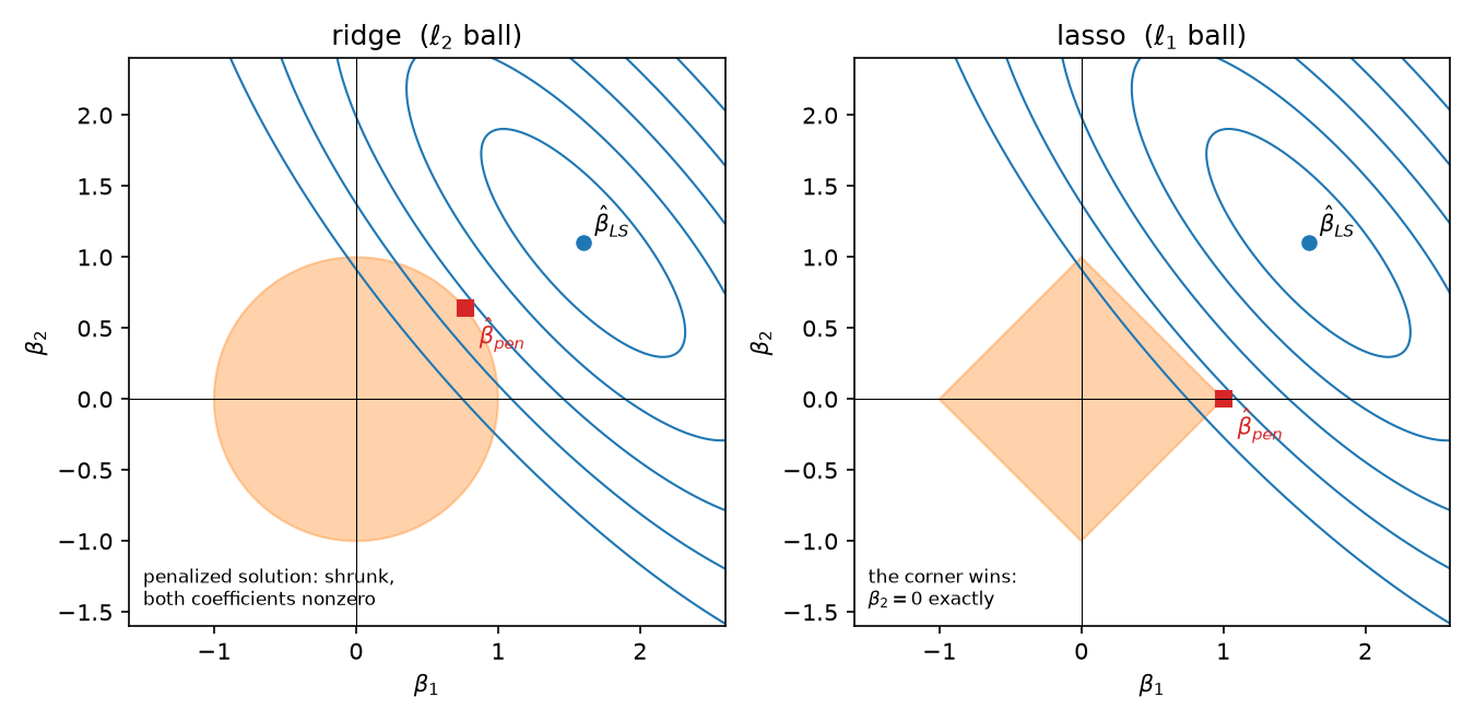
Minimizing the penalized loss is equivalent to minimizing the squared error subject to \(R(\boldsymbol{\beta}) \le\) some budget: the ellipses are contours of the squared error, the shaded region is the penalty ball. The \(\ell_2\) ball is round, so the contours touch it at a generic point with both coefficients nonzero. The \(\ell_1\) ball is a diamond with corners on the axes, and the contours usually hit a corner first – a corner means a coefficient is exactly zero.
LASSO on Ames: the held-out sweep
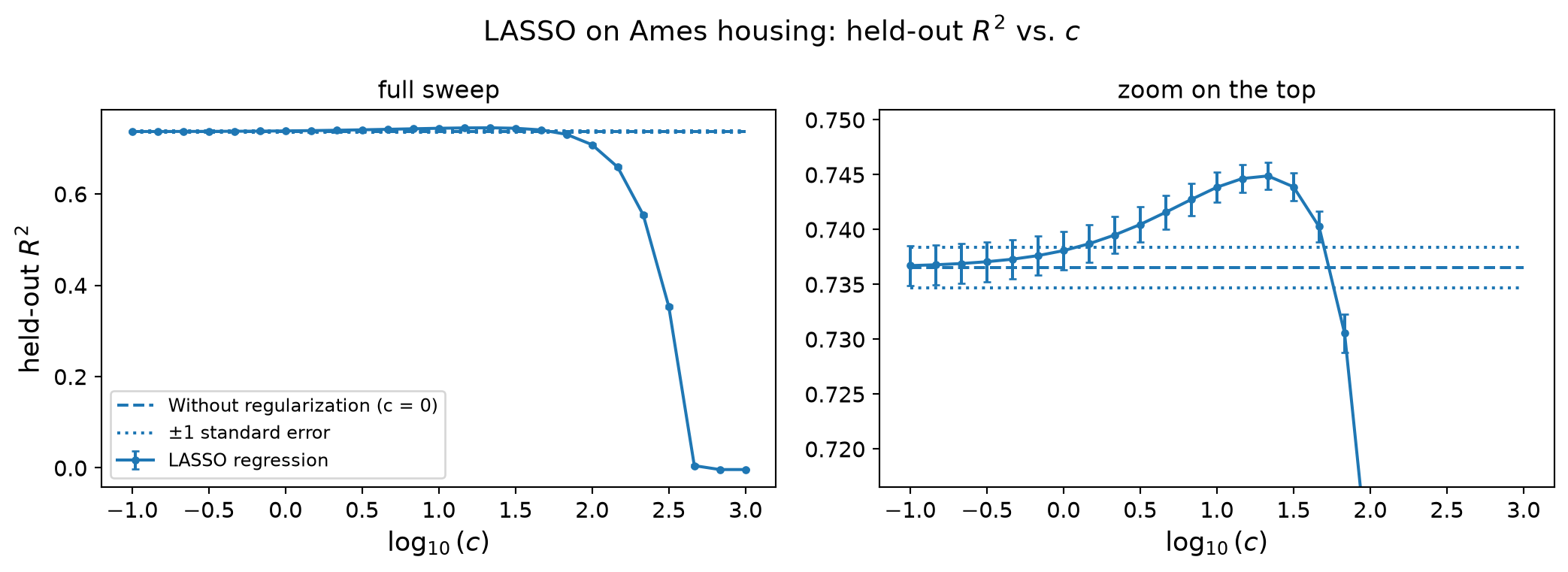
Same protocol as for ridge. sklearn’s Lasso minimizes \(\frac{1}{2n}\Vert X\boldsymbol{\beta}-\mathbf{y}\Vert_2^2 + \alpha\Vert\boldsymbol{\beta}\Vert_1\), so its alpha is \(c/(2n)\); we convert so that the \(c\) axis means the same thing in both plots.
plot_sweep(lasso_scores, 'LASSO regression', 'LASSO on Ames housing: held-out $R^2$ vs. $c$')plt.show()
The shape is the same as for ridge – flat, a modest gain, then collapse – but the collapse comes earlier and is sharper: once \(c\) is large enough to zero the important features, there is nothing left to predict with.
LASSO on Ames: the coefficient path
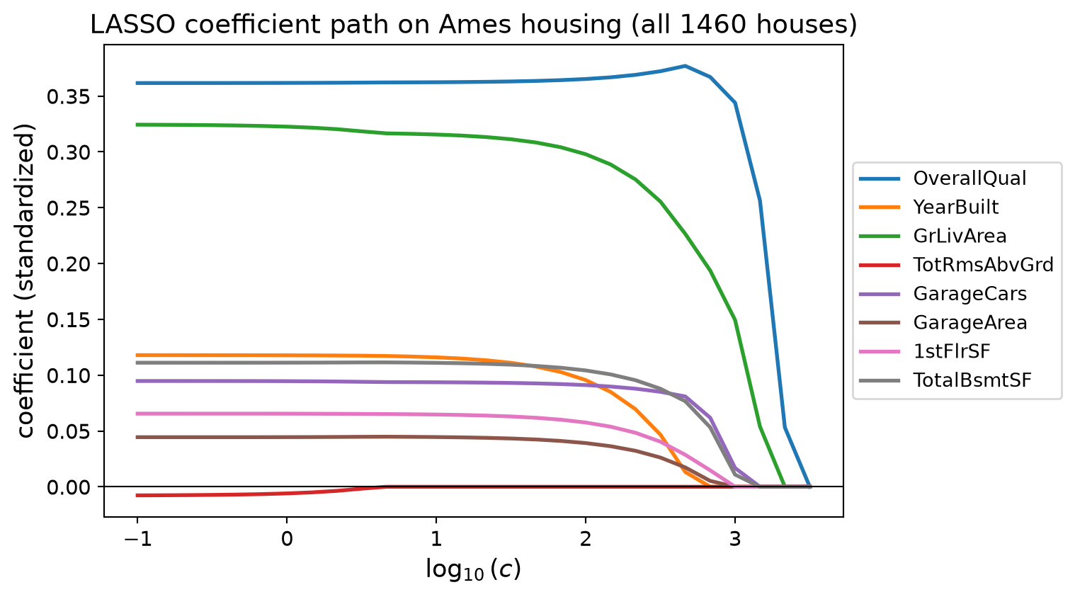
The interesting output is not the \(R^2\) curve but which coefficients survive. For the path we fit the LASSO once on all 1460 (standardized) houses for each \(c\), so the zeros are exact rather than averaged away. Each line is one feature’s coefficient as \(c\) grows.
The one-dimensional formulas say the penalty acts through \(c/n\). The sweep trained on \(n = 292\) houses; the path uses all \(1460\), so the same \(c\) is five times gentler here. Read the path for the order in which coefficients die, not for where the \(c\) values line up with the \(R^2\) plot.
Code
# the coefficients at a few values of c, for reading the pathshow_cs = [0.1, 10, 100, 1000]lasso_path.loc[[c for c in path_cs ifany(np.isclose(c, s, rtol=1e-2) for s in show_cs)]].round(3).T
0.1
10.0
100.0
1000.0
OverallQual
0.362
0.362
0.365
0.344
YearBuilt
0.118
0.116
0.096
0.000
GrLivArea
0.324
0.316
0.298
0.149
TotRmsAbvGrd
-0.008
0.000
0.000
0.000
GarageCars
0.095
0.094
0.091
0.017
GarageArea
0.044
0.045
0.039
0.000
1stFlrSF
0.065
0.065
0.058
0.000
TotalBsmtSF
0.111
0.111
0.104
0.011
Interpretting the coefficient path
With almost no penalty TotRmsAbvGrd has a negative coefficient: “more rooms, lower price, holding living area fixed”. That sign is an artefact of splitting one effect between two near-duplicate columns – the geometry from earlier, in data.
It is the first coefficient LASSO zeroes (by \(c \approx 5\)). Of the pair GrLivArea / TotRmsAbvGrd, LASSO keeps the square footage.
The remaining coefficients shrink slowly until \(c\) is in the hundreds, then YearBuilt goes, followed by GarageArea and 1stFlrSF – the weaker member of each remaining pair. GarageCars and TotalBsmtSF survive them.
By \(c \approx 1000\) two features carry the model, OverallQual and GrLivArea, with a little GarageCars and TotalBsmtSF left.
LASSO did model selection for us: from each collinear pair it kept one column, and it dropped them in the order of how little they added. Ridge would have shrunk every one of these coefficients and set none to zero.
Regularizing the logistic model
The penalty is not special to least squares. Add it to the negative log-likelihood of Lecture 11A and you have regularized logistic regression:
sklearn’s LogisticRegression does this by default: its parameter C is the inverse penalty, \(C = 1/c\), and the default is C=1.0, i.e. an \(\ell_2\) penalty with \(c = 1\). Setting C=np.inf (older versions: penalty=None) gives the plain maximum-likelihood fit of Lecture 11A.
Regularizing the logistic model: admissions
The admissions data of Lecture 11A, three standardized features (the penalty needs it), fit with no penalty, with the default, and with a strong penalty:
Code
df = pd.read_csv(data_file('data/ats-admissions.csv')) # the admissions data of Lecture 11AX_adm = df[['gre', 'gpa', 'rank']]X_adm_s = StandardScaler().fit_transform(X_adm)fits = {'no penalty: C=inf': LogisticRegression(C=np.inf), # older sklearn: penalty=None'default: C=1 (c=1)': LogisticRegression(),'C=0.01 (c=100)': LogisticRegression(C=0.01),}logit_coefs = pd.DataFrame( {name: model.fit(X_adm_s, df['admit']).coef_[0] for name, model in fits.items()}, index=X_adm.columns)logit_coefs.round(3)
no penalty: C=inf
default: C=1 (c=1)
C=0.01 (c=100)
gre
0.265
0.263
0.148
gpa
0.295
0.292
0.148
rank
-0.528
-0.521
-0.233
With \(n = 400\) and three well-conditioned, standardized features, the default penalty barely moves the coefficients – the data dominate \(c = 1\).
Turn the penalty up (\(c = 100\)) and every coefficient is shrunk toward zero, roughly halved; the model becomes less confident everywhere.
The practical point: unless you ask for penalty=None, sklearn is regularizing, and C is \(1/c\) – smallerC means more penalty. In today’s activity you will turn this knob the other way: an \(\ell_1\) penalty on the logistic model, to cut the attributes down to a short list.
Recap: what you can now do
Diagnose multicollinearity: explain why near-dependent columns make the coefficients large and unstable, and read the condition number \(\kappa(X)\) (above \(1000\) is severe).
Penalize the coefficients: ridge shrinks by \(1/(1 + c/s)\) and never reaches zero; LASSO soft-thresholds to exact zeros, so it selects variables.
Follow the two rules: standardize before penalizing (scaler fit on the training split), and choose \(c\) on held-out data. In sklearn’s LogisticRegression, C is \(1/c\) and the penalty is on by default.
For this lecture’s class activity you will diagnose multicollinearity (condition number, bootstrap instability of the OLS coefficients), trace ridge and LASSO paths, choose \(\alpha\) by cross-validation, see what happens without standardizing, and build a short list with an \(\ell_1\)-penalized logistic regression.