Recap: Regularization

DS701 Session 14 — Wed Oct 21, 2026

Today’s plan

• 5 min — knowledge-check review
• 20 min — highlights and Q&A (answer or pass — answering always earns credit)
• 40 min — case study: which attributes the credit union’s loan officers should check
• wrap-up and cold-call check-ins

Knowledge-Check Review

KC 1: Why the coefficients blow up, and two ways to stop them

When two columns of the design matrix are nearly linearly dependent (multicollinearity), the least-squares coefficients tend to become very large in magnitude. Explain in a sentence or two why that happens, how ridge regression’s penalty \(c\Vert\boldsymbol{\beta}\Vert_2^2\) addresses it, and what LASSO’s \(c\Vert\boldsymbol{\beta}\Vert_1\) penalty does that ridge cannot.

KC 2: Reading a condition number

Fitting the Longley data, statsmodels warned that the condition number is about \(10^8\). Define \(\kappa(X)\) in terms of singular values. What does a huge value mean for the fitted coefficients \(\hat{\boldsymbol{\beta}}\), and what does it not mean for the fitted values? Why should you not compute \(\hat{\boldsymbol{\beta}}\) by forming and inverting \(X^\top X\)?

KC 3: Why standardize before penalizing?

Before running ridge or LASSO the lecture standardized every column of \(X\). Plain least squares never needed that. Explain why a penalized fit does, and what LASSO is likely to do to a genuinely useful feature stored in units that make its numbers very small (say, income in millions of dollars) if you skip the step.

Highlights

Regularization: a penalty that trades bias for variance

Lecture 07: flexible fits chase noise → high variance. Regularization is the knob:

\[ \min_{\boldsymbol{\beta}} \Vert X\boldsymbol{\beta} - \mathbf{y}\Vert_2^2 + c\,R(\boldsymbol{\beta}) \]

• Ridge: \(R = \Vert\boldsymbol{\beta}\Vert_2^2\), closed form \((X^\top X + cI)^{-1}X^\top\mathbf{y}\) — always exists, always unique, even with multicollinearity.
• LASSO: \(R = \Vert\boldsymbol{\beta}\Vert_1\).
• \(c = 0\): least squares. \(c \to \infty\): \(\boldsymbol{\beta} \to 0\). In between: fit vs. size — bias bought, variance sold.

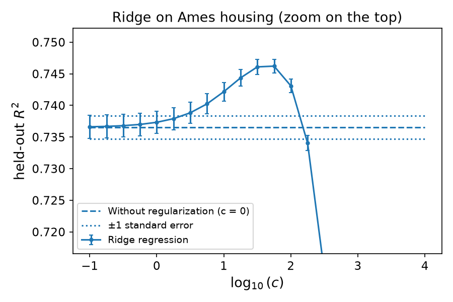
Ames housing, ridge (8 features with three collinear pairs, 100 random splits): held-out \(R^2\) rises with \(c\), then collapses — the sweet spot is found by cross-validation.

Why the coefficients blow up

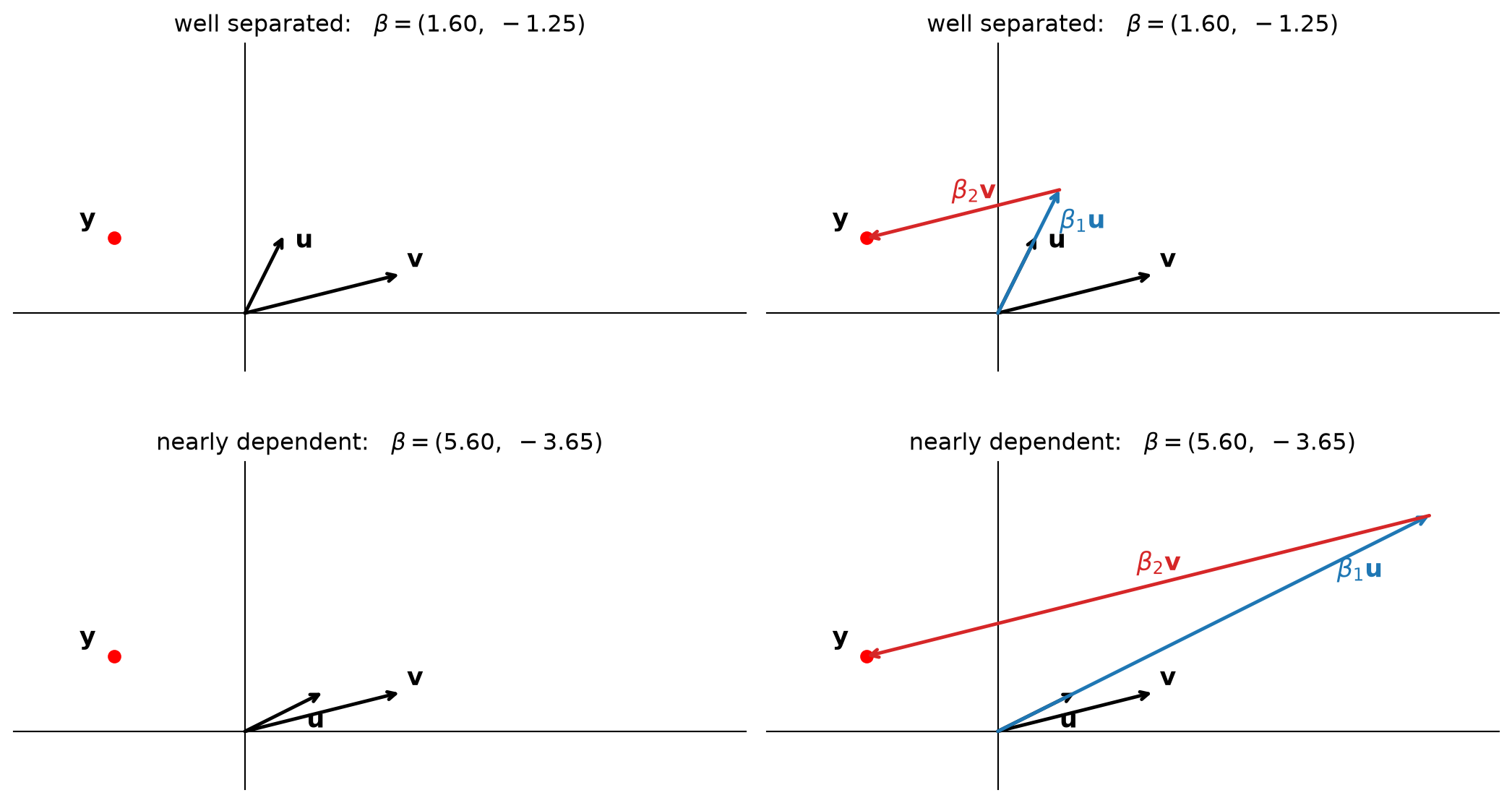
Same \(\mathbf{y}\); nearly parallel columns need \(\boldsymbol{\beta} = (5.60, -3.65)\) instead of \((1.60, -1.25)\).

• Near-dependent columns ⇒ \(\sigma_{\min} \approx 0\) ⇒ huge \(\kappa(X) = \sigma_{\max}/\sigma_{\min}\) (Longley: \(\kappa \approx 10^8\)).
• \(\kappa(X^\top X) = \kappa(X)^2\) — don’t form and invert \(X^\top X\).
• An unstable \(\hat{\boldsymbol{\beta}}\) is variance: refit on a slightly different sample and the coefficients swing.
• Exact dependence: the fit is determined, the coefficients are not. A problem of interpretation, not of prediction.

\(\ell_2\) shrinks, \(\ell_1\) selects

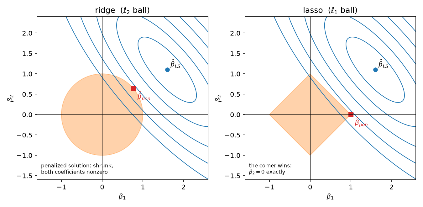
The \(\ell_1\) diamond has corners on the axes; the contours usually hit a corner first, and a corner is an exact zero.

One standardized column, \(s = \mathbf{x}^\top\mathbf{x}\):

\[ \hat\beta_{\text{ridge}} = \frac{\hat\beta_{LS}}{1 + c/s} \]

\[ \hat\beta_{\text{lasso}} = \operatorname{sign}(\hat\beta_{LS})\max\!\big(|\hat\beta_{LS}| - \tfrac{c}{2s},\ 0\big) \]

• Ridge multiplies by a factor in \((0,1)\): small stays small, never zero.
• LASSO subtracts \(c/(2s)\) and stops at zero: any \(|\hat\beta_{LS}|\) below that becomes exactly zero.

LASSO selects the model for you

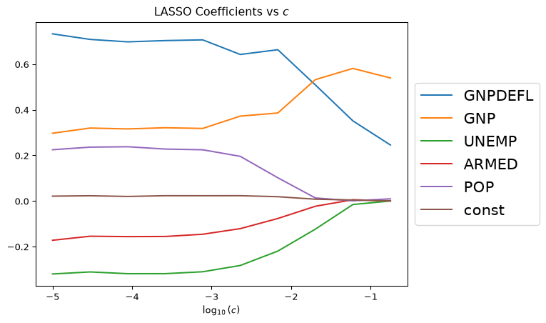
• Ames: as \(c\) grows, TotRmsAbvGrd goes to zero first (its near-duplicate GrLivArea stays), then YearBuilt, GarageArea and 1stFlrSF — from each collinear pair, one column is dropped.
• Ridge would shrink all eight and zero none (until \(c \to \infty\), all at once).
• Instead of searching \(2^p - 1\) subsets, one path — at similar prediction error, with a much more interpretable answer.

Two rules you must not skip

1. Standardize first. The penalty is on the size of \(\boldsymbol{\beta}\). A useful feature in tiny units needs a huge coefficient and gets punished for it; a noise feature in huge units is nearly free. Plain least squares did not care about units — the coefficients absorbed them; a penalized fit does. Standardize \(X\) (fit the scaler on the training split), centre \(\mathbf{y}\), don’t penalize the intercept.
2. Choose \(c\) on held-out data. Training error is always lowest at \(c = 0\) — the penalty can only make the training fit worse. Cross-validate. (And know what CV optimizes: prediction error, not sparsity.)

Today’s activity, Part 2: coefficient paths for both penalties on data where you know which features matter, CV to pick \(\alpha\), and one fit where you “forget” to standardize and watch the lasso throw away a real feature.

Regularizing the logistic model

\[ \min_{\boldsymbol{\beta}}\; -\ell(\boldsymbol{\beta}) + c\Vert\boldsymbol{\beta}\Vert_2^2 \qquad\text{or}\qquad -\ell(\boldsymbol{\beta}) + c\Vert\boldsymbol{\beta}\Vert_1 \]

• The penalty is not special to least squares: add it to 11A’s negative log-likelihood.
• sklearn’s LogisticRegression() does this by default: \(\ell_2\), C=1.0, and \(C = 1/c\) — smaller C = more penalty.
• C=np.inf (older versions: penalty=None) gives back the plain MLE fit of 11A.
• Same two rules: standardize, pick C by CV.

Admissions, standardized features:

	no penalty	C=1	C=0.01
gre	0.265	0.263	0.148
gpa	0.295	0.292	0.148
rank	−0.528	−0.521	−0.233

\(n = 400\): the default barely moves anything; \(c = 100\) roughly halves every coefficient.

Where this goes next

• \(\kappa(X) = \sigma_{\max}/\sigma_{\min}\) used the singular values of \(X\) without ever saying what they are. Next lecture — the SVD — is the tool underneath: it explains why \(X^\top X\) squares the conditioning problem, why ridge is “shrink each singular direction by \(\sigma_j^2/(\sigma_j^2 + c)\)”, and how the same decomposition gives low-rank compression and, later, PCA.
• Regularization comes back unchanged for neural networks (weight decay).

In-Class Activity

Activity — Case Study 11B: Which Attributes Should the Loan Officers Check?

The client: the same credit union’s small-business lending desk.

• Our loan officers can verify only a few applicant attributes by hand — which ones?
• Why do the model’s weights on some attributes swing from one fit to the next?

The data: a simulator of the desk’s applicants, whose true answer you know

• Member records cannot be shared — this is a prototype until they can be

Activity — The Parts

1. Diagnose: the condition number of the desk’s attribute matrix; refit OLS on bootstrap resamples and watch the copied-column coefficients swing
2. Ridge vs lasso: coefficient paths on attributes that are correlated, irrelevant, or stored in the wrong units; pick \(\alpha\) by CV; see what forgetting to standardize costs
3. The short list: an L1-penalized logistic regression on the approval outcome

Report out: a memo to the desk — which attributes to check, and the one caveat they must hear.

Activity — Logistics

• Work in groups of 2–3. Open your section’s notebook.
• Parts marked (autograded) are submitted to Gradescope; the rest is participation.
• Staff will circulate — be ready to explain any part of your work.
• Dependencies: numpy, pandas, matplotlib, scikit-learn.

The activity notebook goes live on the day of the lecture. Colab is optional — you can also open it on GitHub and run it locally.

Going deeper

Full lecture notes: Regularization

• What is regularization? — the penalized least-squares problem
• Condition Number — \(\kappa(X)\), \(\kappa(X^\top X) = \kappa(X)^2\), and Longley: reading the condition number
• Why the coefficients blow up — the geometry of nearly parallel columns
• Ridge Regression — the closed form, the 1-D estimator, Scaling
• The LASSO — the soft threshold, coefficient path on the Ames data; Model Selection
• Regularizing the logistic model — sklearn’s C = 1/c
• Previous: Logistic Regression (Lecture 11A)
• Background: bias–variance in Generalization; the normal equations in Linear Regression