Recap: SVD and Low-Rank Approximation
DS701 Session 15 — Mon Oct 26, 2026
One factorization, three ways to read it
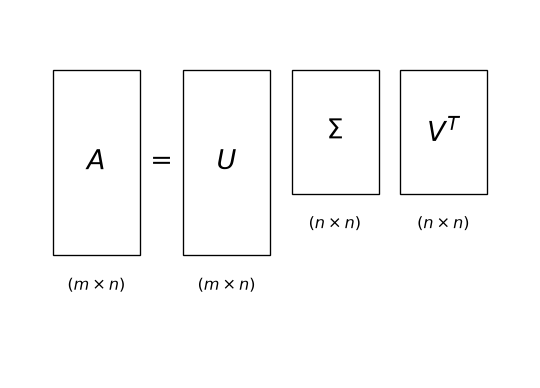
\[A = U\Sigma V^T, \qquad A\mathbf{v}_i = \sigma_i \mathbf{u}_i\]
- As matrices — orthonormal \(U\) (left singular vectors), diagonal \(\Sigma\) (singular values, sorted, \(\ge 0\)), orthonormal \(V\) (right singular vectors).
- As a map — \(A\) sends each \(\mathbf{v}_i\) to \(\mathbf{u}_i\), stretched by \(\sigma_i\); the \(\mathbf{v}_i\) beyond the rank go to zero.
- As a sum — \(A = \sum_i \sigma_i \mathbf{u}_i\mathbf{v}_i^T\): rank-1 layers, weighted by \(\sigma_i\), heaviest first.
Always exists; the \(\sigma_i\) are unique, the vectors unique up to sign. np.linalg.svd(A, full_matrices=False) returns U, s, Vt — note the transpose and that s is a vector.
The spectrum is an importance ranking
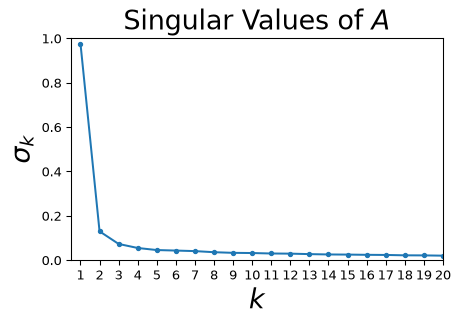
Traffic matrix, \(1008\times121\), rank 121.
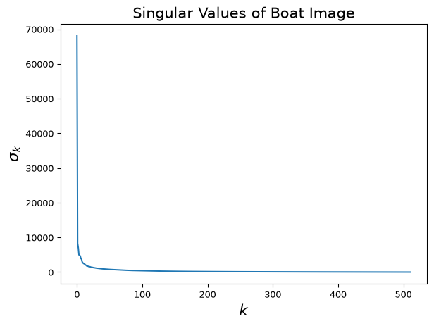
Boat photo, \(512\times512\), rank 512 (log scale: \(\sigma_1\) is \(8\times\) \(\sigma_2\)).
Both are full rank; both have a sharp elbow. Everything after the elbow is a rank-1 layer with a tiny weight — the matrix is close to rank 5, or 40: low effective rank. Occam’s razor, measured: a few hidden patterns carry most of the data.
Eckart–Young: the best rank-\(k\) approximation
Distance between matrices: Frobenius, \(\lVert A - B\rVert_F = \sqrt{\sum_{ij}(a_{ij}-b_{ij})^2}\) — Euclidean distance in \(\mathbb{R}^{mn}\).
- \(A^{(k)} = \arg\min_{\operatorname{rank} B = k} \lVert A - B\rVert_F\) is the truncated SVD: first \(k\) columns of \(U\) and \(V\), top-left \(k\times k\) of \(\Sigma\).
- Its error is exactly the tail: \(\lVert A - A^{(k)}\rVert_F^2 = \sum_{i=k+1}^{n}\sigma_i^2\).
- Best among all rank-\(k\) matrices — however cleverly built — and for every \(k\) from one decomposition.
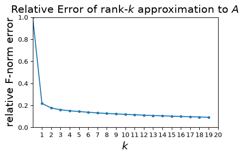
Relative error read straight off the singular values: 9% at \(k=20\).
Layers of a photograph
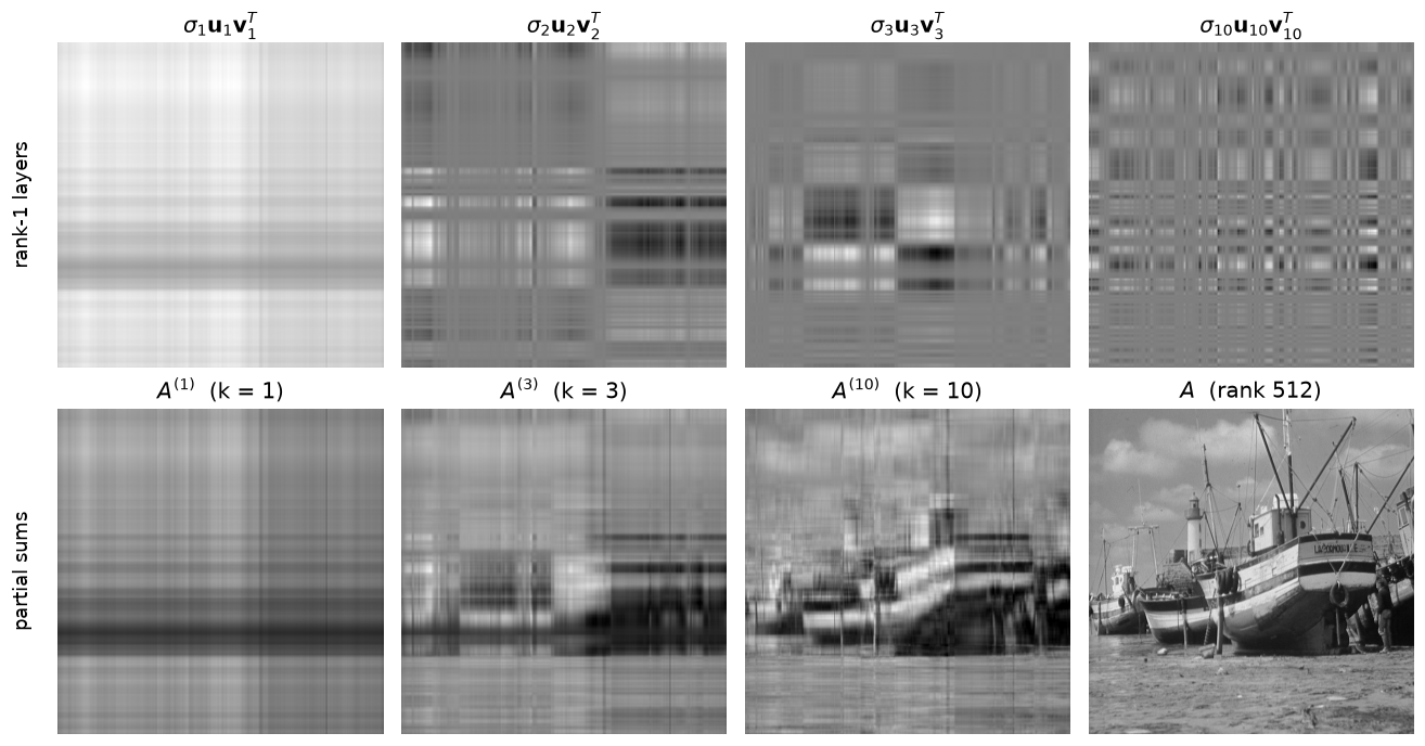
Top row: individual rank-1 layers \(\sigma_i\mathbf{u}_i\mathbf{v}_i^T\) — each is a row profile times a column profile. Bottom row: partial sums. Ten layers already give the boats; the remaining 502 add texture. Today you rebuild a photo at \(k = 1, 5, 20, 50\) and put numbers on this.
Compression: what you keep, what you pay

Rank 40 of 512:
- store \(U'\), \(\Sigma'\), \(V'\): \(40\,(512 + 512 + 1) = 41{,}000\) numbers vs \(262{,}144\) — a 6.4× compression;
- relative Frobenius error \(\approx 8\%\);
- what is lost: the layers with the smallest weights — fine texture, low-contrast detail.
Same arithmetic for the traffic matrix: \(20\,(1008+121)\) vs \(1008\cdot121\) — 81% smaller, 9% error.
Two readings of a low-rank matrix
Common patterns — columns of \(U\).
\(\mathbf{a}_j \approx \sum_{i\le k} \sigma_i v_{ij}\mathbf{u}_i\) (\(v_{ij}\) = entry \(j\) of \(\mathbf{v}_i\)): every column of the data is a mix of the same \(k\) patterns; \(\mathbf{u}_1\) is the strongest one (traffic: the daily rhythm shared by all 121 traces).
Latent factors — rows of \(U\Sigma\) and columns of \(V^T\).
\(a_{ij} = \tilde U_{i,:}\cdot \tilde V_{:,j}\): user \(i\) and item \(j\) are both points in \(\mathbb{R}^k\), and the entry is their inner product. Netflix: \(k \approx 20\).
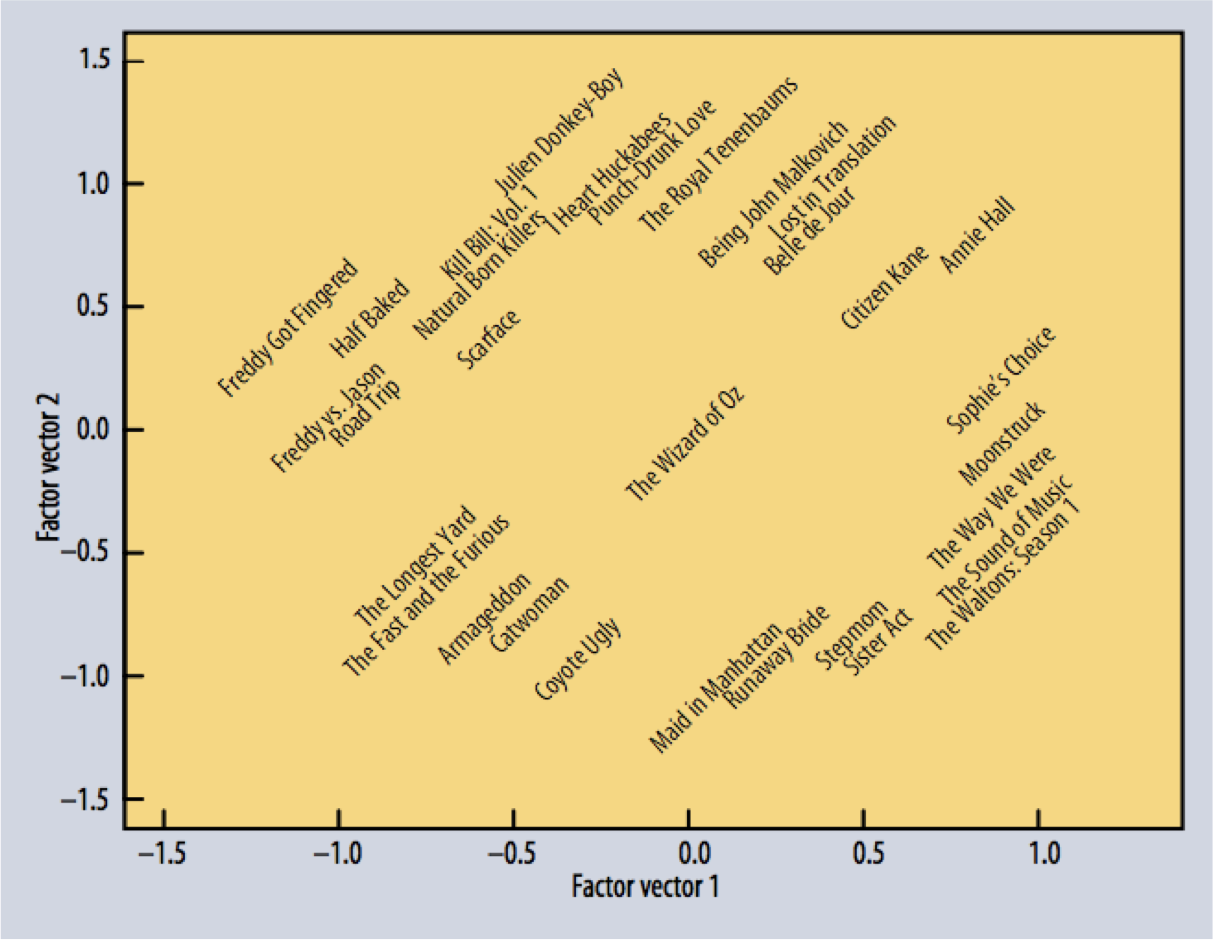
Movies placed by their two strongest latent factors — nobody typed in genres. Source: Koren et al., IEEE Computer, 2009.
Activity — Case Study 12: How Much Can a Trail-Camera Network Compress Its Photos?
Goal: an environmental nonprofit uploads wildlife trail-camera photos over a metered cellular link and asks how far a photo can be compressed before a biologist can no longer identify the animal — and what “rank” means for their budget. On a stand-in frame (a scikit-learn sample photo, not theirs) you take the image apart with np.linalg.svd and rebuild it (Part 1), verify \(\Sigma^2 = \operatorname{eig}(A^TA)\) and rank = number of non-zero singular values (Part 2), rebuild it at rank 1, 5, 20 and 50 (Part 3), price each rank in Frobenius error, energy and compression ratio (Part 4), and check Eckart–Young against two rank-20 competitors (Part 5). You close with a two-sentence memo to the nonprofit: the rank you would set, and the kind of photo it would fail on.
- Work in groups of 2–3.
- Parts marked (autograded) are submitted to Gradescope; the rest is participation.
- Staff will circulate — be ready to explain any part of your work.
- Dependencies:
numpy,pandas,matplotlib,scikit-learn.


The activity notebook goes live on the day of the lecture. Colab is optional — you can also open it on GitHub and run it locally.