DS701 Session 21 — Mon Nov 16, 2026
Write down the three pieces of the TF-IDF weight of a term \(t\) in a document \(d\) — term frequency, inverse document frequency, and how they combine — and say in one sentence what kind of term ends up with a large weight. What weight does a term that appears in every document of the corpus get, and why is that the point?
The lecture notes that with one-hot encodings the similarity of two different words is always 0, while word embeddings put words with similar meanings close together (small angle, high cosine). Explain why the sparse representations — one-hot, bag of words, TF-IDF — can never express that “doctor” and “physician” are related, and what an embedding does differently that makes it possible.
A static embedding (Word2Vec) gives “bank” one vector; a contextual model (BERT) gives “bank” a different vector in “river bank” and in “bank account”. Using the lecture’s description of attention (queries, keys, values, softmax-weighted sum), explain what mechanism lets the second vector depend on the neighbouring words. Then name one task from the lecture where that difference matters and one where a static embedding is good enough.
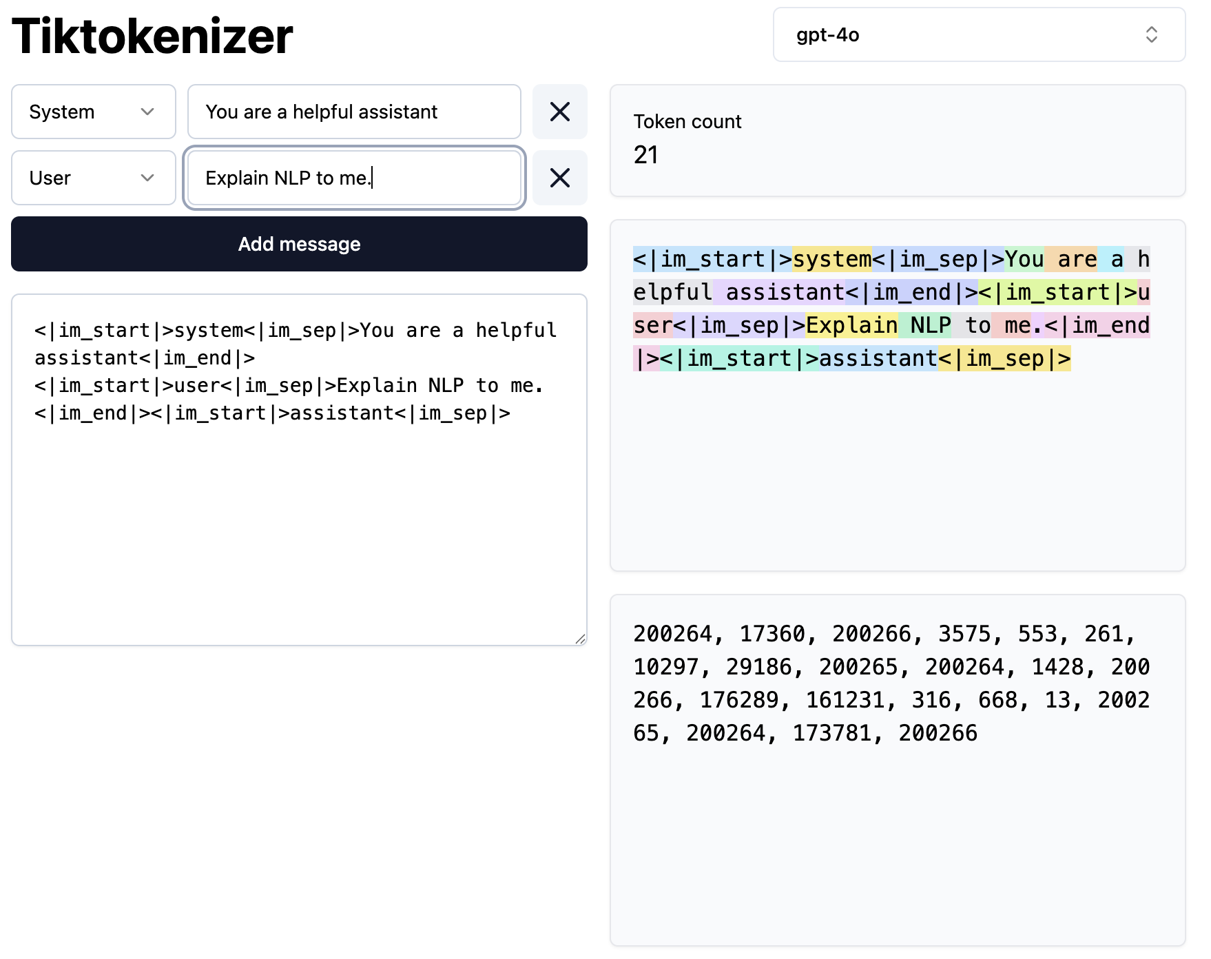
Models cannot read strings. Every NLP system, from a 1990s search engine to GPT, starts the same way:
token, ##ize. Normalize as you go (lowercase, …).
Today’s activity builds steps 1–3 by hand and checks every number against scikit-learn.
Throw away order and grammar; keep how many times each vocabulary word occurs. A document becomes a vector in \(\mathbb{R}^V\):
| the | cat | sat | on | mat | dog | log | emu | |
|---|---|---|---|---|---|---|---|---|
| “The cat sat on the mat.” | 2 | 1 | 1 | 1 | 1 | 0 | 0 | 0 |
| “The dog sat on the log.” | 2 | 0 | 1 | 1 | 0 | 1 | 1 | 0 |
| “The emu sat on the mat.” | 2 | 0 | 1 | 1 | 1 | 0 | 0 | 1 |
the; sat, on are identical across rows. Raw counts mostly say “this is English”.cat, dog, emu) are the smallest entries — count 1.\[ \text{tf-idf}(t,d) \;=\; \underbrace{\mathrm{tf}(t,d)}_{\text{frequent here}}\;\times\;\underbrace{\log\frac{N}{\mathrm{df}(t)}}_{\text{rare overall}} \qquad \mathrm{df}(t) = \#\{\text{documents containing } t\} \]
the, sat, on have \(\mathrm{df}=3 \Rightarrow \mathrm{idf}=0\); cat has \(\mathrm{df}=1 \Rightarrow \mathrm{idf}=\log 3\); mat has \(\mathrm{df}=2 \Rightarrow \log 1.5\). The document vector is now carried by cat, dog, emu, mat, log.TfidfVectorizer is not the textbook formula. Its defaults:
\[ \mathrm{idf}_{\text{sk}}(t) = \log\frac{1+N}{1+\mathrm{df}(t)} + 1, \qquad\text{then each document row is divided by its } \ell_2 \text{ norm.} \]
the can still top the ranking — the lecture’s table shows the = 0.709 in every row.stop_words="english", min_df / max_df to prune the vocabulary, sublinear_tf for \(1+\log\mathrm{tf}\). On thousands of documents the smoothing barely matters; on three it does.\[ \cos\theta = \frac{v_1\cdot v_2}{\lVert v_1\rVert\,\lVert v_2\rVert} \]
The blind spot.
“my laptop will not power on” “notebook fails to boot”
share no term after stop-word removal → cosine exactly 0, however similar the meaning. Sparse lexical vectors see overlap, not synonymy.
Sparse (one-hot, BoW, TF-IDF): one axis per word, all axes orthogonal, similarity = literal overlap. Vocabulary-sized and mostly zeros.
Dense embedding: a learned vector of a few hundred dimensions per word; similar meaning ⇒ small angle. Individual coordinates are not interpretable; the geometry is (king − man + woman ≈ queen).
The bridge you already know — LSA. Take the SVD of the TF-IDF matrix (Lecture 12) and keep the top \(k\) directions (Lecture 13): each direction is a combination of terms that co-occur across documents, and projecting a document onto them gives a dense \(k\)-vector. “laptop” and “notebook” load on the same direction, so the two tickets now score \(>0\). Today’s stretch section does exactly this.
| static (Word2Vec, GloVe) | contextual (BERT, GPT) | |
|---|---|---|
| per word | one vector | one per occurrence |
| “bank” | same vector | river ≠ account |
| how learned | shallow net predicts word ↔︎ context | deep transformer |
| size / cost | 100–300 d, cheap | 768+ d, GPU |
| good for | similarity, clustering | ambiguity, NER, QA, translation |
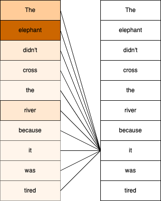
“The elephant didn’t cross the river because it was tired.”
For each token, in parallel over the whole sequence:
\[\text{Attention}(Q,K,V) = \mathrm{softmax}\!\left(\frac{QK^\top}{\sqrt{d_k}}\right)V\]
The weights are computed from the input — that is what makes the embedding contextual, and what neither TF-IDF nor Word2Vec nor LSA can do. Encoder-only (BERT) reads both ways for understanding; decoder-only (GPT) predicts the next token for generation.
| Need | Reach for | Where |
|---|---|---|
| tokenize, count, TF-IDF, cosine, LSA | sklearn.feature_extraction.text, TruncatedSVD |
today’s activity |
| classical text processing, corpora, sentiment lexicons | NLTK | A5 — NLP Packages |
production pipelines: POS, parsing, NER, displacy |
spaCy | A5, lecture NER section |
| topic modeling with transformer embeddings (embed → UMAP → HDBSCAN → c-TF-IDF) | BERTopic | A5, lecture |
| tokenizers and pre-trained transformer models | Hugging Face transformers |
lecture |
| applications on top of LLMs | LangChain | A5 |
Notice how much of the BERTopic pipeline you already own: dimensionality reduction (L13), density clustering (L3–4), TF-IDF per cluster (today). The transformer only supplies step 1.
Goal: build the text pipeline by hand — tokenizer, bag-of-words matrix, TF, IDF, TF-IDF — checking each against CountVectorizer / TfidfVectorizer; then use cosine similarity to retrieve the nearest document. Stretch: measure retrieval accuracy on real newsgroup posts, hit TF-IDF’s blind spot (a same-meaning pair scoring exactly 0), and close it with LSA — TruncatedSVD on the TF-IDF matrix — before asking what a transformer embedding would add.
numpy, pandas, matplotlib, scikit-learn — no spaCy / NLTK / transformer downloads (the one optional cell that uses them is clearly marked).The activity notebook goes live on the day of the lecture. Colab is optional — you can also open it on GitHub and run it locally.
Full lecture notes: Natural Language Processing