
| admit | gre | gpa | rank | |
|---|---|---|---|---|
| 0 | 0 | 380 | 3.61 | 3 |
| 1 | 1 | 660 | 3.67 | 3 |
| 2 | 1 | 800 | 4.00 | 1 |
| 3 | 1 | 640 | 3.19 | 4 |
| 4 | 0 | 520 | 2.93 | 4 |
| 5 | 1 | 760 | 3.00 | 2 |
| 6 | 1 | 560 | 2.98 | 1 |
| 7 | 0 | 400 | 3.08 | 2 |
| 8 | 1 | 540 | 3.39 | 3 |
| 9 | 0 | 700 | 3.92 | 2 |
Logistic Regression and Regularization



Introduction
So far we have seen linear regression:
- a continuous valued observation is estimated as a linear (or affine) function of the independent variables.
Now we will look at the following situation.
Estimating a Probability
Imagine that you are observing a binary variable – value 0 or 1.
That is, these could be pass/fail, admit/reject, Democrat/Republican, etc.
Assume there is some probability of observing a 1, and that probability is a function of certain independent variables.
So the key properties of a problem that make it appropriate for logistic regression are:
- You are trying to predict a categorical variable
- You want to estimate a probability of seeing a particular value of the categorical variable.
Example: Grad School Admission
Note
The following example was adapted from this URL which seems to be no longer available. There is an archive of the page and an archive of the dataset.
Let’s consider this question:
What is the probability I will be admitted to Grad School?
Let’s see how variables, such as,
- GRE (Graduate Record Exam scores),
- GPA (grade point average), and
- prestige of the undergraduate institution
affect admission into graduate school.
The response variable, admit/don’t admit, is a binary variable.
So there are three predictor variables: gre, gpa and rank.
- We will treat the variables gre and gpa as continuous.
- The variable rank takes on the values 1 through 4 with 1 being the highest prestige.
Let’s look at 10 lines of the data:
Code
df.shape(400, 4)and some summary statistics:
Code
df.describe()| admit | gre | gpa | rank | |
|---|---|---|---|---|
| count | 400.000000 | 400.000000 | 400.000000 | 400.00000 |
| mean | 0.317500 | 587.700000 | 3.389900 | 2.48500 |
| std | 0.466087 | 115.516536 | 0.380567 | 0.94446 |
| min | 0.000000 | 220.000000 | 2.260000 | 1.00000 |
| 25% | 0.000000 | 520.000000 | 3.130000 | 2.00000 |
| 50% | 0.000000 | 580.000000 | 3.395000 | 2.00000 |
| 75% | 1.000000 | 660.000000 | 3.670000 | 3.00000 |
| max | 1.000000 | 800.000000 | 4.000000 | 4.00000 |
We can also plot histograms of the variables:
Code
df.hist(figsize = (10, 4));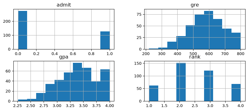
Note how
df.hist()automatically plots a histogram for each column in the dataframe as a subplot.
Let’s look at how each independent variable affects admission probability by plotting the mean admission probability as a function of the independent variable.
Note that there’s a greatly expanded
groupbysection in the Pandas refresher.
We add error bars to the means to indicate the standard error of the mean.
First, rank:
Code
import numpy as np

# Calculate mean and standard error
grouped = df.groupby('rank')['admit']
means = grouped.mean()

# Compute 'standard error of the mean'
errors = grouped.std() / np.sqrt(grouped.count())

# Plot with error bars
ax = means.plot(marker='o', yerr=errors, fontsize=12, capsize=5)
ax.set_ylabel('P[admit]', fontsize=16)
ax.set_xlabel('Rank', fontsize=16);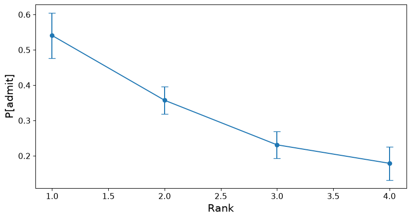
Next, GRE:
Code
grouped_gre = df.groupby('gre')['admit']
means_gre = grouped_gre.mean()
errors_gre = grouped_gre.std() / np.sqrt(grouped_gre.count())

ax = means_gre.plot(marker='o', yerr=errors_gre, fontsize=12, capsize=5)
ax.set_ylabel('P[admit]', fontsize=16)
ax.set_xlabel('GRE', fontsize=16);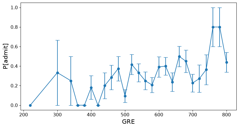
Finally, GPA (for this visualization, we aggregate GPA into 8 bins):
Code
bins = np.linspace(df.gpa.min(), df.gpa.max(), 8)
bin_centers = (bins[:-1] + bins[1:]) / 2
grouped_gpa = df.groupby(np.digitize(df.gpa, bins)).mean()['admit']
ax = grouped_gpa.plot(marker='o', fontsize=12)
ax.set_ylabel('P[admit]', fontsize=16)
ax.set_xlabel('GPA', fontsize=16)
ax.set_xticks(range(1, len(bin_centers) + 1))
ax.set_xticklabels([f'{center:.2f}' for center in bin_centers], rotation=45);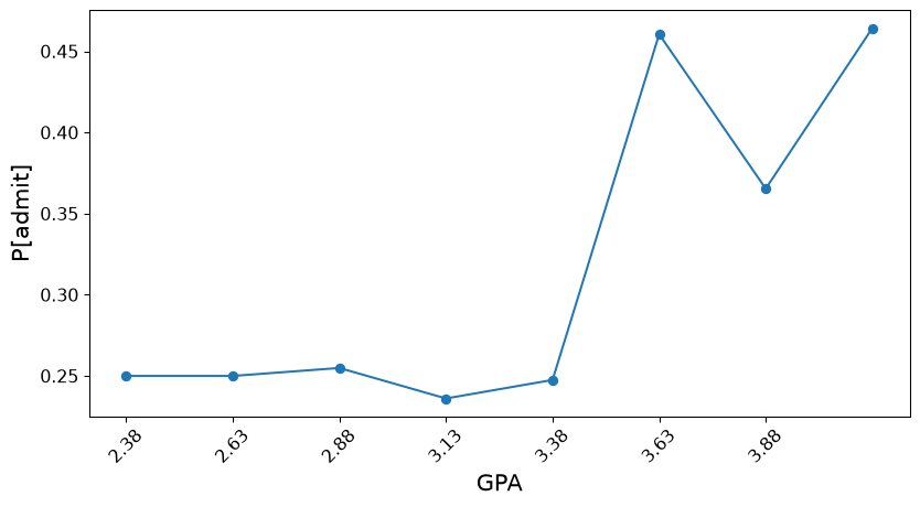
Finally, we plot admission status versus GRE score for each data point for each of the four ranks:
Code
df1 = df[df['rank']==1]
df2 = df[df['rank']==2]
df3 = df[df['rank']==3]
df4 = df[df['rank']==4]

fig = plt.figure(figsize = (10, 5))

ax1 = fig.add_subplot(221)
df1.plot.scatter('gre','admit', ax = ax1)
plt.title('Rank 1 Institutions')

ax2 = fig.add_subplot(222)
df2.plot.scatter('gre','admit', ax = ax2)
plt.title('Rank 2 Institutions')

ax3 = fig.add_subplot(223, sharex = ax1)
df3.plot.scatter('gre','admit', ax = ax3)
plt.title('Rank 3 Institutions')

ax4 = fig.add_subplot(224, sharex = ax2)
plt.title('Rank 4 Institutions')
df4.plot.scatter('gre','admit', ax = ax4);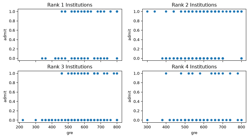
What we want to do is to fit a model that predicts the probability of admission as a function of these independent variables.
Logistic Regression
Logistic regression is concerned with estimating a probability.
However, all that is available are categorical observations, which we will code as 0/1.
That is, these could be pass/fail, admit/reject, Democrat/Republican, etc.
Now, a linear function like \(\beta_0 + \beta_1 x\) cannot be used to predict probability directly, because
- the linear function takes on all values (from -\(\infty\) to +\(\infty\)),
- and probability only ranges over \([0, 1]\).
Odds and Log-Odds
However, there is a transformation of probability that works: it is called log-odds.
For any probabilty \(p\), the odds is defined as \(p/(1-p)\), which is the ratio of the probability of an event to the probability of the non-event.
Notice that odds vary from 0 to \(\infty\), and odds < 1 indicates that \(p < 1/2\).
Now, there is a good argument that to fit a linear function, instead of using odds, we should use log-odds.
That is simply \(\log p/(1-p)\) which is also called the logit function, which is an abbreviation for logistic unit.
Code
pvec = np.linspace(0.01, 0.99, 100)
ax = plt.figure(figsize = (6, 4)).add_subplot()
ax.plot(pvec, np.log(pvec / (1-pvec)))
ax.tick_params(labelsize=12)
ax.set_xlabel('Probability', fontsize = 14)
ax.set_ylabel('Log-Odds', fontsize = 14)
ax.set_title('Logit Function: $\log (p/1-p)$', fontsize = 16);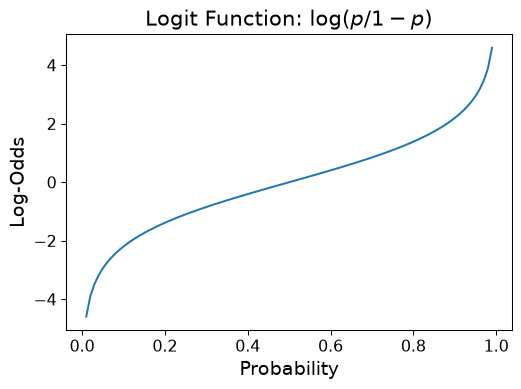
So, logistic regression does the following: it does a linear regression of \(\beta_0 + \beta_1 x\) against \(\log p/(1-p)\).
That is, it fits:
\[ \begin{aligned} \beta_0 + \beta_1 x &= \log \frac{p(x)}{1-p(x)} \\ e^{\beta_0 + \beta_1 x} &= \frac{p(x)}{1-p(x)} \quad \text{(exponentiate both sides)} \\ e^{\beta_0 + \beta_1 x} (1-p(x)) &= p(x) \quad \text{(multiply both sides by $1-p(x)$)} \\ e^{\beta_0 + \beta_1 x} &= p(x) + p(x)e^{\beta_0 + \beta_1 x} \quad \text{(distribute $p(x)$)} \\ \frac{e^{\beta_0 + \beta_1 x}}{1 +e^{\beta_0 + \beta_1 x}} &= p(x) \end{aligned} \]
So, logistic regression fits a probability of the following form:
\[ p(x) = P(y=1\mid x) = \frac{e^{\beta_0+\beta_1 x}}{1+e^{\beta_0+\beta_1 x}}. \]
This is a sigmoid function; when \(\beta_1 > 0\),
- as \(x\rightarrow \infty\), then \(p(x)\rightarrow 1\) and
- as \(x\rightarrow -\infty\), then \(p(x)\rightarrow 0\).
Holding \(\beta_0\) constant, we see that as \(\beta_1\) increases, the logistic function becomes steeper.
Code
alphas = [-4, -8,-12,-20]
alphas = [-8, -8, -8, -8]
betas = [0.2,0.4,0.6,1]
x = np.arange(40)
fig = plt.figure(figsize=(8, 6))
ax = plt.subplot(111)

for i in range(len(alphas)):
    a = alphas[i]
    b = betas[i]
    y = np.exp(a+b*x)/(1+np.exp(a+b*x))
#     plt.plot(x,y,label=r"$\frac{e^{%d + %3.1fx}}{1+e^{%d + %3.1fx}}\;\beta_0=%d, \beta_1=%3.1f$" % (a,b,a,b,a,b))
    ax.plot(x,y,label=r"$\beta_0=%d,$    $\beta_1=%3.1f$" % (a,b))
ax.tick_params(labelsize=12)
ax.set_xlabel('x', fontsize = 14)
ax.set_ylabel('$p(x)$', fontsize = 14)
ax.legend(loc='center left', bbox_to_anchor=(1, 0.5), prop={'size': 16})
ax.set_title('Logistic Functions', fontsize = 16);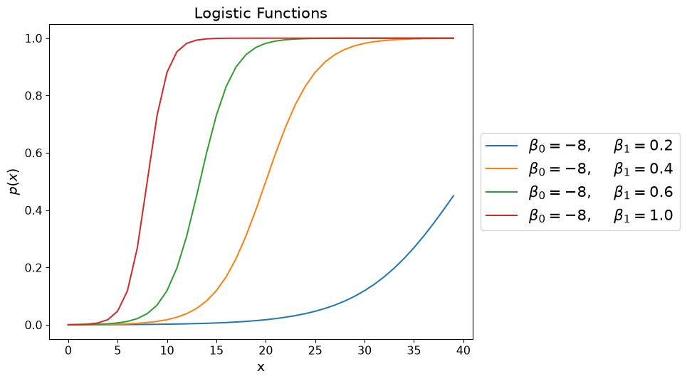
Holding \(\beta_1\) constant, we see that as \(\beta_0\) increases, the logistic function shifts to the right.
Code
alphas = [-4, -8,-12,-20]
betas = [0.4, 0.4, 0.4, 0.4]
x = np.arange(40)
fig = plt.figure(figsize=(8, 6))
ax = plt.subplot(111)

for i in range(len(alphas)):
    a = alphas[i]
    b = betas[i]
    y = np.exp(a+b*x)/(1+np.exp(a+b*x))
#     plt.plot(x,y,label=r"$\frac{e^{%d + %3.1fx}}{1+e^{%d + %3.1fx}}\;\beta_0=%d, \beta_1=%3.1f$" % (a,b,a,b,a,b))
    ax.plot(x,y,label=r"$\beta_0=%d,$    $\beta_1=%3.1f$" % (a,b))
ax.tick_params(labelsize=12)
ax.set_xlabel('x', fontsize = 14)
ax.set_ylabel('$p(x)$', fontsize = 14)
ax.legend(loc='center left', bbox_to_anchor=(1, 0.5), prop={'size': 16})
ax.set_title('Logistic Functions', fontsize = 16);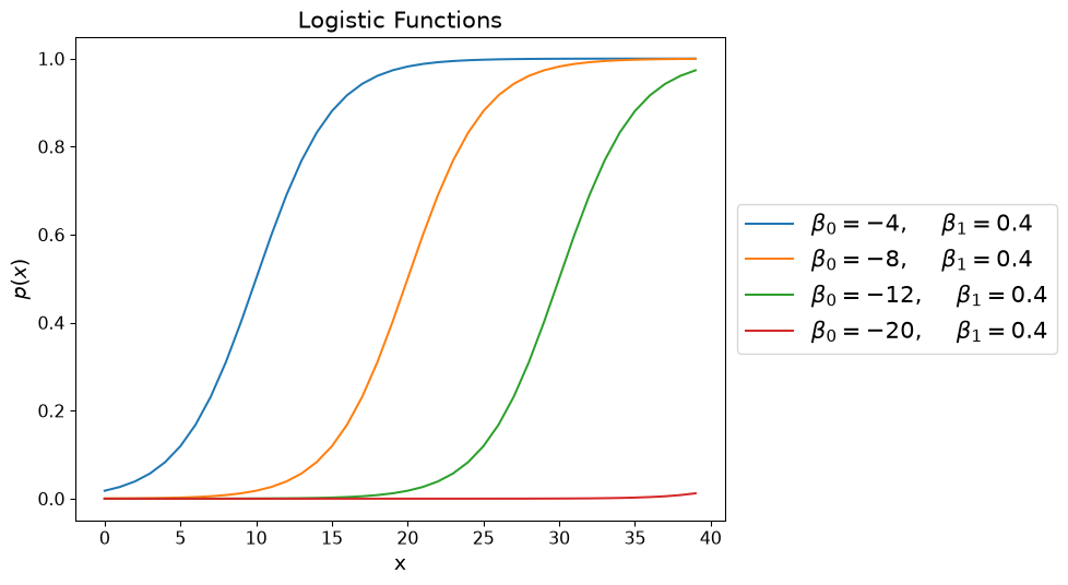
Varying both \(\beta_0\) and \(\beta_1\) gives us a more general logistic function.
Code
alphas = [-4, -8,-12,-20]
betas = [0.2,0.4,0.6,1]
x = np.arange(40)
fig = plt.figure(figsize=(8, 6))
ax = plt.subplot(111)

for i in range(len(alphas)):
    a = alphas[i]
    b = betas[i]
    y = np.exp(a+b*x)/(1+np.exp(a+b*x))
#     plt.plot(x,y,label=r"$\frac{e^{%d + %3.1fx}}{1+e^{%d + %3.1fx}}\;\beta_0=%d, \beta_1=%3.1f$" % (a,b,a,b,a,b))
    ax.plot(x,y,label=r"$\beta_0=%d,$    $\beta_1=%3.1f$" % (a,b))
ax.tick_params(labelsize=12)
ax.set_xlabel('x', fontsize = 14)
ax.set_ylabel('$p(x)$', fontsize = 14)
ax.legend(loc='center left', bbox_to_anchor=(1, 0.5), prop={'size': 16})
ax.set_title('Logistic Functions', fontsize = 16);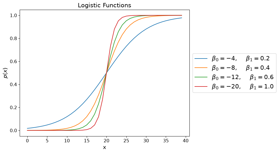
Parameter \(\beta_1\) controls how fast \(p(x)\) raises from \(0\) to \(1\)
The value of -\(\beta_0\)/\(\beta_1\) shows the value of \(x\) for which \(p(x)=0.5\)
Another interpretation of \(\beta_0\) is that it gives the base rate – the unconditional probability of a 1.
That is, if you knew nothing about a particular data item, then \(p(x) = 1/(1+e^{-\beta_0})\).
Code
# plot the base rate as a function of beta_0
beta_0_values = np.linspace(-10, 10, 100)
base_rate = 1 / (1 + np.exp(-beta_0_values))
plt.figure(figsize=(6, 4))
plt.plot(beta_0_values, base_rate)
plt.xlabel('beta_0')
plt.ylabel('Base Rate')
plt.title('Base Rate as a function of beta_0')
plt.show()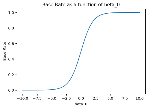
The function \(f(x) = \log (x/(1-x))\) is called the logit function.
So a compact way to describe logistic regression is that it finds regression coefficients \(\beta_0, \beta_1\) to fit:
\[ \text{logit}\left(p(x)\right)=\log\left(\frac{p(x)}{1-p(x)} \right) = \beta_0 + \beta_1 x. \]
Note also that the inverse logit function is:
\[ \text{logit}^{-1}(x) = \frac{e^x}{1 + e^x}. \]
Somewhat confusingly, this is called the logistic function.
So, the best way to think of logistic regression is that we compute a linear function:
\[ \beta_0 + \beta_1 x, \]
and then map that to a probability using the inverse \(\text{logit}\) function:
\[ \frac{e^{\beta_0+\beta_1 x}}{1+e^{\beta_0+\beta_1 x}}. \]
Logistic vs Linear Regression
Let’s take a moment to compare linear and logistic regression.
In Linear regression we fit
\[ y_i = \beta_0 +\beta_1 x_i + \epsilon_i. \]
We do the fitting by minimizing the sum of squared errors \(\Vert\epsilon\Vert\). This can be done in closed form using either geometric arguments or by calculus.
Now, if \(\epsilon_i\) comes from a normal distribution with mean zero and some fixed variance, then minimizing the sum of squared errors is exactly the same as finding the maximum likelihood of the data with respect to the probability of the errors.
So, in the case of linear regression, it is a lucky fact that the MLE of \(\beta_0\) and \(\beta_1\) can be found by a closed-form calculation.
In Logistic regression we fit
\[ \text{logit}(p(x_i)) = \beta_0 + \beta_1 x_i. \]
with \(\text{P}(y_i=1\mid x_i)=p(x_i).\)
How should we choose parameters?
Here too, we use Maximum Likelihood Estimation of the parameters.
That is, we choose the parameter values that maximize the likelihood of the data given the model.
\[ \text{P}(y_i \mid x_i) = \left\{\begin{array}{lr}\text{logit}^{-1}(\beta_0 + \beta_1 x_i)& \text{if } y_i = 1\\ 1 - \text{logit}^{-1}(\beta_0 + \beta_1 x_i)& \text{if } y_i = 0\end{array}\right. \]
We can write this as a single expression:
\[ \text{P}(y_i \mid x_i) = \text{logit}^{-1}(\beta_0 + \beta_1 x_i)^{y_i} (1-\text{logit}^{-1}(\beta_0 + \beta_1 x_i))^{1-y_i}, \]
where we assume the parameters are fixed.
We can reinterpret this to express the likelihood of parameters \(\beta_0\), \(\beta_1\):
\[ L(\beta_0, \beta_1 \mid x_i, y_i) = \text{logit}^{-1}(\beta_0 + \beta_1 x_i)^{y_i} (1-\text{logit}^{-1}(\beta_0 + \beta_1 x_i))^{1-y_i}, \]
given that we have observed the data \((x_i, y_i)\).
This is our objective function to maximize.
However, there is no closed-form solution so we optimize it numerically with gradient descent.
How Gradient Descent Works
Algorithm:
Initialize parameters: Start with random values \(\beta^{(0)}\)
Compute gradient: Calculate \(\nabla \ell(\beta^{(t)})\) - the direction of steepest increase
Update parameters: Take a step in that direction: \[\beta^{(t+1)} = \beta^{(t)} + \alpha \nabla \ell(\beta^{(t)})\] where \(\alpha\) is the learning rate (step size)
Repeat steps 2-3 until convergence (gradient \(\approx 0\) or max iterations reached)
Result: Parameters that (locally) maximize the likelihood of the observed data.
Logistic Regression In Practice
So, in summary, we have:
Input pairs \((x_i,y_i)\)
Output parameters \(\widehat{\beta_0}\) and \(\widehat{\beta_1}\) that maximize the likelihood of the data given these parameters for the logistic regression model.
Method Maximum likelihood estimation, obtained by gradient descent.
The standard package will give us a coefficient \(\beta_i\) for each independent variable (feature).
If we want to include a constant (i.e., \(\beta_0\)) we need to add a column of 1s (just like in linear regression).
Code
df['intercept'] = 1.0
train_cols = df.columns[1:]
train_cols
Index(['gre', 'gpa', 'rank', 'intercept'], dtype='str')Code
logit = sm.Logit(df['admit'], df[train_cols])

# fit the model
result = logit.fit()
Optimization terminated successfully.
Current function value: 0.574302
Iterations 6Statsmodels gives us a summary of the model fit.
Code
result.summary()| Dep. Variable: | admit | No. Observations: | 400 |
|---|---|---|---|
| Model: | Logit | Df Residuals: | 396 |
| Method: | MLE | Df Model: | 3 |
| Date: | Mon, 17 Aug 2026 | Pseudo R-squ.: | 0.08107 |
| Time: | 17:09:38 | Log-Likelihood: | -229.72 |
| converged: | True | LL-Null: | -249.99 |
| Covariance Type: | nonrobust | LLR p-value: | 8.207e-09 |
| coef | std err | z | P>|z| | [0.025 | 0.975] | |
|---|---|---|---|---|---|---|
| gre | 0.0023 | 0.001 | 2.101 | 0.036 | 0.000 | 0.004 |
| gpa | 0.7770 | 0.327 | 2.373 | 0.018 | 0.135 | 1.419 |
| rank | -0.5600 | 0.127 | -4.405 | 0.000 | -0.809 | -0.311 |
| intercept | -3.4495 | 1.133 | -3.045 | 0.002 | -5.670 | -1.229 |
Notice that all of our independent variables are considered significant (no confidence intervals contain zero).
Using the Model
Note that by fitting a model to the data, we can make predictions for inputs that were not in the training data.
Furthermore, we can make a prediction of a probability for cases where we don’t have enough data to estimate the probability directly – e.g., for specific parameter values.
Let’s see how well the model fits the data.
We have three independent variables, so in each case we’ll use average values for the two that we aren’t evaluating.
GPA (GRE = 600, Rank = 2.5):
Code
bins = np.linspace(df.gpa.min(), df.gpa.max(), 10)
groups = df.groupby(np.digitize(df.gpa, bins))
prob = [result.predict([600, b, 2.5, 1.0]) for b in bins]
ax = plt.figure(figsize = (7, 4)).add_subplot()
ax.plot(bins, prob)
ax.plot(bins,groups.admit.mean(),'o')
ax.tick_params(labelsize=12)
ax.set_xlabel('gpa', fontsize = 14)
ax.set_ylabel('P[admit]', fontsize = 14)
ax.set_title('Marginal Effect of GPA', fontsize = 16);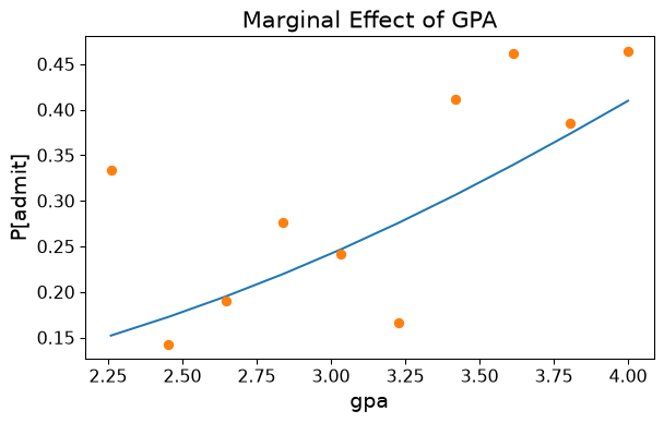
GRE Score (GPA = 3.4, Rank = 2.5):
Code
prob = [result.predict([b, 3.4, 2.5, 1.0]) for b in sorted(df.gre.unique())]
ax = plt.figure(figsize = (7, 4)).add_subplot()
ax.plot(sorted(df.gre.unique()), prob)
ax.plot(df.groupby('gre').mean()['admit'],'o')
ax.tick_params(labelsize=12)
ax.set_xlabel('gre', fontsize = 14)
ax.set_ylabel('P[admit]', fontsize = 14)
ax.set_title('Marginal Effect of GRE', fontsize = 16);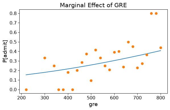
Institution Rank (GRE = 600, GPA = 3.4):
Code
prob = [result.predict([600, 3.4, b, 1.0]) for b in range(1,5)]
ax = plt.figure(figsize = (7, 4)).add_subplot()
ax.plot(range(1,5), prob)
ax.plot(df.groupby('rank').mean()['admit'],'o')
ax.tick_params(labelsize=12)
ax.set_xlabel('Rank', fontsize = 14)
ax.set_xlim([0.5,4.5])
ax.set_ylabel('P[admit]', fontsize = 14)
ax.set_title('Marginal Effect of Rank', fontsize = 16);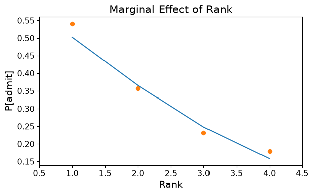
Logistic Regression in Perspective
At the start of lecture we emphasized that logistic regression is concerned with estimating a probability model for discrete (0/1) data.
However, it may well be the case that we want to do something with the probability that amounts to classification.
For example, we may classify data items using a rule such as “Assign item \(x_i\) to Class 1 if \(p(x_i) > 0.5\)”.
For this reason, logistic regression could be considered a classification method.
Let’s use our logistic regression as a classifier.
We want to ask whether we can correctly predict whether a student gets admitted to graduate school.
Let’s separate our training and test data:
Code
X_train, X_test, y_train, y_test = model_selection.train_test_split(
        df[train_cols], df['admit'],
        test_size=0.4, random_state=1)
Now, there are some standard metrics used when evaluating a binary classifier.
Let’s say our classifier is outputting “yes” when it thinks the student will be admitted.
There are four cases:
- Classifier says “yes”, and student is admitted: True Positive.
- Classifier says “yes”, and student is not admitted: False Positive.
- Classifier says “no”, and student is admitted: False Negative.
- Classifier says “no”, and student is not admitted: True Negative.
Precision is the fraction of “yes” classifications that are correct:
\[ \mbox{Precision} = \frac{\mbox{True Positives}}{\mbox{True Positives + False Positives}}. \]
Recall is the fraction of admits that we say “yes” to:
\[ \mbox{Recall} = \frac{\mbox{True Positives}}{\mbox{True Positives + False Negatives}}. \]
Code
def evaluate(y_train, X_train, y_test, X_test, threshold):

    # learn model on training data
    logit = sm.Logit(y_train, X_train)
    result = logit.fit(disp=False)

    # make probability predictions on test data
    y_pred = result.predict(X_test)

    # threshold probabilities to create classifications
    y_pred = y_pred > threshold

    # report metrics
    precision = metrics.precision_score(y_test, y_pred)
    recall = metrics.recall_score(y_test, y_pred)
    return precision, recall

precision, recall = evaluate(y_train, X_train, y_test, X_test, 0.5)

print(f'Precision: {precision:0.3f}, Recall: {recall:0.3f}')
Precision: 0.586, Recall: 0.340Now, let’s get a sense of average accuracy:
Code
PR = []
for i in range(20):
    X_train, X_test, y_train, y_test = model_selection.train_test_split(
            df[train_cols], df['admit'],
            test_size=0.4)
    PR.append(evaluate(y_train, X_train, y_test, X_test, 0.5))
Code
avgPrec = np.mean([f[0] for f in PR])
avgRec = np.mean([f[1] for f in PR])
print(f'Average Precision: {avgPrec:0.3f}, Average Recall: {avgRec:0.3f}')
Average Precision: 0.632, Average Recall: 0.211Sometimes we would like a single value that describes the overall performance of the classifier.
For this, we take the harmonic mean of precision and recall, called F1 Score:
\[ \mbox{F1 Score} = 2 \;\;\frac{\mbox{Precision} \cdot \mbox{Recall}}{\mbox{Precision} + \mbox{Recall}}. \]
Using this, we can evaluate other settings for the threshold.
Code
import warnings
warnings.filterwarnings("ignore")
def evalThresh(df, thresh):
    PR = []
    for i in range(20):
        X_train, X_test, y_train, y_test = model_selection.train_test_split(
                df[train_cols], df['admit'],
                test_size=0.4)
        PR.append(evaluate(y_train, X_train, y_test, X_test, thresh))
    avgPrec = np.mean([f[0] for f in PR])
    avgRec = np.mean([f[1] for f in PR])
    return 2 * (avgPrec * avgRec) / (avgPrec + avgRec), avgPrec, avgRec

tvals = np.linspace(0.05, 0.8, 50)
f1vals = [evalThresh(df, tval)[0] for tval in tvals]
Code
plt.figure(figsize=(6, 3))
plt.plot(tvals,f1vals)
plt.ylabel('F1 Score')
plt.xlabel('Threshold for Classification')
plt.title('F1 as a function of Threshold');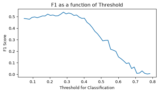
Based on this plot, we can say that the best classification threshold appears to be around 0.3, where precision and recall are:
Code
F1, Prec, Rec = evalThresh(df, 0.3)
print('Best Precision: {:0.3f}, Best Recall: {:0.3f}'.format(Prec, Rec))
Best Precision: 0.420, Best Recall: 0.671The example here is based on http://blog.yhathq.com/posts/logistic-regression-and-python.html where you can find additional details.
ROC-AUC Curve
The ROC-AUC curve is a plot of the true positive rate against the false positive rate at various threshold settings.
The AUC is the area under the ROC curve.
The AUC is a measure of the overall performance of the classifier.
Code
# Get predicted probabilities from the model
y_pred_proba = result.predict(df[train_cols])

# Compute ROC curve and AUC
fpr, tpr, thresholds = metrics.roc_curve(df['admit'], y_pred_proba)
auc_score = metrics.roc_auc_score(df['admit'], y_pred_proba)

# Plot ROC curve
fig, ax = plt.subplots(figsize=(4, 4))
ax.plot(fpr, tpr, linewidth=2, label=f'ROC curve (AUC = {auc_score:.3f})')
ax.plot([0, 1], [0, 1], 'k--', linewidth=1, label='Random classifier')
ax.set_xlabel('False Positive Rate', fontsize=12)
ax.set_ylabel('True Positive Rate', fontsize=12)
ax.set_title('ROC Curve for Logistic Regression Model', fontsize=14)
ax.legend(loc='lower right', fontsize=11)
ax.grid(True, alpha=0.3)
ax.tick_params(labelsize=11)
plt.tight_layout()
plt.show()

print(f"AUC Score: {auc_score:.4f}")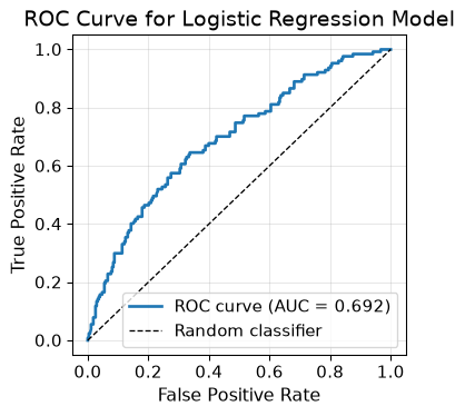
AUC Score: 0.6921Recap
- Logistic regression is used to predict a probability.
- It is a linear model for the log-odds.
- It is fit by maximum likelihood.
- It can be evaluated as a classifier.
From logistic regression to regularization
- We can now fit linear models (last lecture) and logistic models (just now), both by choosing coefficients \(\boldsymbol{\beta}\) that minimize a loss.
- Both can overfit, exactly as Generalization warned: with many (or correlated) features, the fitted \(\boldsymbol{\beta}\) chases noise in the training set and generalizes poorly.
- Regularization is the fix – add a penalty on the size of \(\boldsymbol{\beta}\) to the loss – and it is the same idea for linear regression, logistic regression, and later neural networks.
- Part 2 develops it for linear regression, where the geometry is easiest to see.
Part 2: Regularization
Overfitting
We have referenced the concept of overfitting previously in our generalization and decision tree lectures.
We know that a model that overfits does not generalize well. In other words, the model does not perform well on data it was not trained on.
We observe overfitting when the training accuracy of the model is high, while the accuracy on the validation set (or held out test set) stagnates.
In this part of the lecture we will discuss regularization. A technique to help prevent overfitting. We will see how to apply regularization to regression problems.
However, regularization is a general technique to ensure models learn broad patterns and is applicable in neural networks.
What is regularization?
We know regularization is a way to prevent overfitting, but how does this actually work?
The idea behind regularization is to penalize a model’s loss function during training. The added penalty will discourage the model from becoming too complex (i.e., overfitting).
In regression, our training process was to compute coefficients \(\boldsymbol{\beta}\) by minimizing
\[ \min_{\boldsymbol{\beta}} \Vert X \boldsymbol{\beta} - \mathbf{y}\Vert_{2}^{2}, \]
where \(X\in\mathbb{R}^{m\times n}\) is the design matrix and \(\mathbf{y}\in\mathbb{R}^{m}\) are the dependent variables.
Regularization adds a function \(R(\boldsymbol{\beta})\) to the minimization problem. A regularized minimization problem is then: compute \(\boldsymbol{\beta}\) such that
\[ \min_{\boldsymbol{\beta}} \Vert X \boldsymbol{\beta} - \mathbf{y}\Vert_{2}^{2} + cR(\boldsymbol{\beta}). \]
The regularization coefficient \(c\) is a hyperparameter that controls the importance of the regularization term \(R(\boldsymbol{\beta})\).
We will consider two common forms of \(R(\boldsymbol{\beta})\):
- \(R(\boldsymbol{\beta}) = \Vert \boldsymbol{\beta}\Vert_{2}^{2}\), called ridge regression, and
- \(R(\boldsymbol{\beta}) = \Vert \boldsymbol{\beta}\Vert_1\), called LASSO regression.
Overview
In this part of the lecture we will cover:
- situations where regression is needed to help
- when to use the different types of regression
- importance of the hyperparameter \(c\)
Multicollinearity
In statistics, multicollinearity (also collinearity) is a phenomenon in which two or more predictor variables in a multiple regression model are highly correlated, meaning that one can be linearly predicted from the others with a substantial degree of accuracy.
We will see that multicollinearity can be problematic in our regression models.
To address these issues, we will consider
- What are the potential sources for multicollinearity?
- What does multicollinearity tell us about our data?
Understanding these questions will inform us how regularization can be used to mitigate the issue of multicollinearity.
Sources of Multicollinearity
We will be working with our design matrix \(X\in\mathbb{R}^{m\times n}\), where each row corresponds to an instance of data and the \(n\) columns are the \(n\) features of the data points.
We will see that multicollinearity arises when the columns of \(X\) are linearly dependent (or nearly linearly dependent).
As a consequence, the matrix \(X^{T}X\) is no longer invertible. However, as we saw in our Linear Regression lecture, the least squares solution still exists. It is just not unique.
What are the situations where this can happen?
One clear case is when \(m < n\), which means \(X\) has more columns than rows. That is, there are more features than there are observations in the data.
However, we can still observe multicollinearity when \(m > n\).
This can happen when the columns of \(X\) happen to be linearly dependent because of the nature of the data itself. In particular, this happens when one column is a linear function of the other columns. This means that one independent variable is a linear function of one or more of the others.
Unfortunately, in practice we will run into trouble even if variables are almost linearly dependent.
To illustrate the multcollinearity problem, we’ll load a standard dataset.
The Longley dataset contains various US macroeconomic variables from 1947–1962.
We have the following features:
- GNP - GNP (Gross National Product)
- GNPDEFL - GNP deflator
- UNEMP - Number of unemployed
- ARMED - Size of armed forces
- POP - Population
- YEAR - Year (1947 - 1962)
We want to predict:
- TOTEMP - Total Employment
Code
from statsmodels.datasets.longley import load_pandas
y = load_pandas().endog
X = load_pandas().exog
X['const'] = 1.0
X.index = X['YEAR']
y.index = X['YEAR']
X.drop('YEAR', axis = 1, inplace = True)
print("X.head()")
print(X.head())
print("\n\ny.head()")
print(y.head())
X.head()
GNPDEFL GNP UNEMP ARMED POP const
YEAR
1947.0 83.0 234289.0 2356.0 1590.0 107608.0 1.0
1948.0 88.5 259426.0 2325.0 1456.0 108632.0 1.0
1949.0 88.2 258054.0 3682.0 1616.0 109773.0 1.0
1950.0 89.5 284599.0 3351.0 1650.0 110929.0 1.0
1951.0 96.2 328975.0 2099.0 3099.0 112075.0 1.0
y.head()
YEAR
1947.0 60323.0
1948.0 61122.0
1949.0 60171.0
1950.0 61187.0
1951.0 63221.0
Name: TOTEMP, dtype: float64An important warning is issued stating the condition number is large. What does this mean?
Code
ols_model = sm.OLS(y, X)
ols_results = ols_model.fit()
with warnings.catch_warnings():
    warnings.simplefilter('ignore')
    print(ols_results.summary())
OLS Regression Results
==============================================================================
Dep. Variable: TOTEMP R-squared: 0.987
Model: OLS Adj. R-squared: 0.981
Method: Least Squares F-statistic: 156.4
Date: Mon, 17 Aug 2026 Prob (F-statistic): 3.70e-09
Time: 17:09:41 Log-Likelihood: -117.83
No. Observations: 16 AIC: 247.7
Df Residuals: 10 BIC: 252.3
Df Model: 5
Covariance Type: nonrobust
==============================================================================
coef std err t P>|t| [0.025 0.975]
------------------------------------------------------------------------------
GNPDEFL -48.4628 132.248 -0.366 0.722 -343.129 246.204
GNP 0.0720 0.032 2.269 0.047 0.001 0.143
UNEMP -0.4039 0.439 -0.921 0.379 -1.381 0.573
ARMED -0.5605 0.284 -1.975 0.077 -1.193 0.072
POP -0.4035 0.330 -1.222 0.250 -1.139 0.332
const 9.246e+04 3.52e+04 2.629 0.025 1.41e+04 1.71e+05
==============================================================================
Omnibus: 1.572 Durbin-Watson: 1.248
Prob(Omnibus): 0.456 Jarque-Bera (JB): 0.642
Skew: 0.489 Prob(JB): 0.725
Kurtosis: 3.079 Cond. No. 1.21e+08
==============================================================================
Notes:
[1] Standard Errors assume that the covariance matrix of the errors is correctly specified.
[2] The condition number is large, 1.21e+08. This might indicate that there are
strong multicollinearity or other numerical problems.Condition Number
The notion of conditioning pertains to the perturbation behavior of a mathematical problem. A well-conditioned problem is one where small changes to the inputs produce small changes to the output. An ill-conditioned problem is one where small changes in the input can produce very large changes in the output.
The condition number of a matrix provides an indication of how accurately you can compute with it.
A large condition number tells us that our problem is ill conditioned, i.e., small changes to the input can produce very large changes in the output.
A small condition number tells us that our problem is well-conditioned.
The condition number is derived using matrix norms, which is beyond the scope of this course. However, we will use the following definition for the condition number of our matrix
\[ \kappa(X) = \frac{\sigma_{\text{max}}}{\sigma_{\text{min}}}, \]
where \(\sigma_{\text{max}}\), \(\sigma_{\text{min}}\) are the maximum and minimum singular values, respectively, of the design matrix \(X\).
The SVD again provides us with important properties of a matrix.
Another important fact is that
\[ \kappa(X^TX) = \frac{\sigma_{\text{max}}^2}{\sigma_{\text{min}}^2}. \]
This means that if we have a poorly conditioned data matrix \(X\), then \(X^TX\) is even more poorly conditioned.
This is why you should never work directly with \(X^TX\) as it can be numerically unstable.
Normal Equations
To solve the least-squares problem we solve the normal equations
\[ X^TX\boldsymbol{\beta} = X^Ty. \]
These equations always have at least one solution. However, the at least one part is problematic.
If there are multiple solutions, they are in a sense all equivalent in that they yield the same value of \(\Vert X\boldsymbol{\beta} - y\Vert_2\).
However, the actual values of \(\boldsymbol{\beta}\) can vary tremendously and so it is not clear how best to interpret which solution is actually the best.
When does this problem occur?
Linear Dependence
It occurs when \(X^TX\) is not invertible.
This happens when the columns of \(X\) are linearly dependent – that is, one column can be expressed as a linear combination of the other columns.
In that case, it is not possible to solve the normal equations by computing \(\hat{\boldsymbol{\beta}} \neq (X^TX)^{-1}X^Ty.\)
This is the simplest kind of multicollinearity.
What are the implications of a matrix not being invertible on the condition number?
If a matrix \(Z = X^{T}X\) is not invertible, there is a zero singular value. This implies
\[ \kappa(Z) = \infty. \]
In other words, the problem of solving an equation with a non-invertible matrix is completely ill-conditioned. In fact, it’s a problem that is impossible to solve.
Near Linear Dependence
Near linear dependence causes problems as well. This can happen, for example, due to measurement errors. Or when two or more columns are strongly correlated.
In such a situation, we have some column of our design matrix that is close to being a linear combination of the other columns.
When these situations occur we will have problems with linear regression.
As a result of near linear dependence, the smallest singular value of the design matrix \(X\) will be close to zero. This means that \(\kappa(X)\) will be very large.
The condition number tells us that a small change in the input to our problem can result in large changes to the output.
This means that for a design matrix \(X\) with near linearly dependent columns, the values we compute for \(\boldsymbol{\beta}\) in our linear regression can vary significantly.
This is why we see the addition of a regularization (penalty) term involving \(\boldsymbol{\beta}\) in the least squares minimization problem. This process regularizes the solution \(\boldsymbol{\beta}\).
Longley Dataset
Recall that the condition number of our data is around \(10^8\).
A large condition number is evidence of a problem.
As a general rule of thumb:
- If the condition number is less than 100, there is no serious problem with multicollinearity.
- Condition numbers between 100 and 1000 imply moderate to strong multicollinearity.
- Condition numbers bigger than 1000 indicate severe multicollinearity.
Let’s look at pairwise scatter plots of the Longley data.
Code
sns.pairplot(X[['GNPDEFL', 'GNP', 'UNEMP', 'ARMED', 'POP']])
plt.show()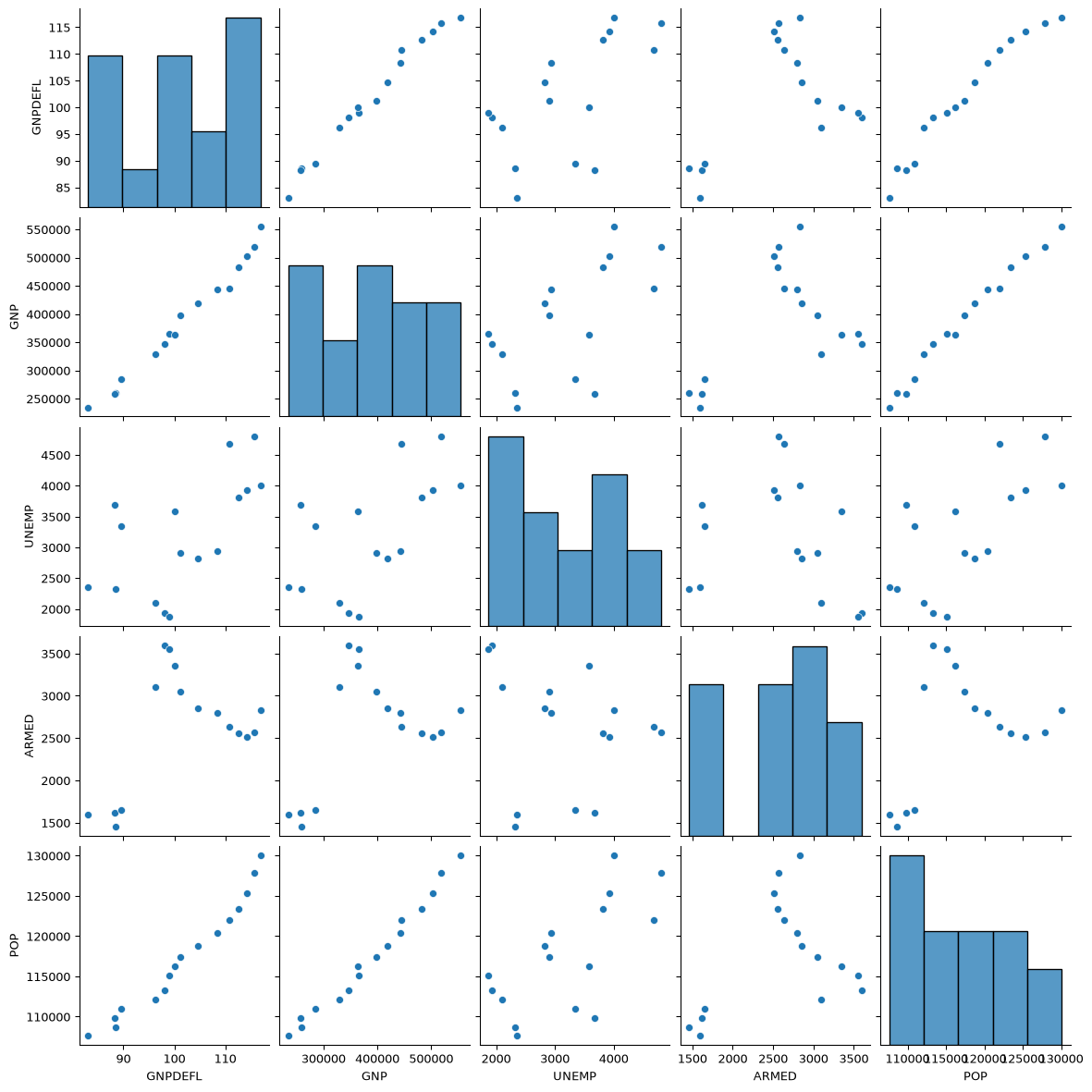
We can see very strong linear relationships between, e.g., GNP Deflator, GNP, and Population.
Addressing Multicollinearity
Here are two strategies we can employ to address multicollinearity:
- Ridge Regression
- Model Selection via LASSO
PCA also addresses multicollinearity by transforming the correlated features into uncorrelated features. However in this approach you lose the original features, which is less explainable.
Ridge Regression
The first thing to note is that when columns of \(X\) are nearly dependent, the components of \(\hat{\boldsymbol{\beta}}\) tend to be large in magnitude.
Code
ax = ut.plotSetup(size=(4,2))
ut.centerAxes(ax)
u = np.array([1, 2])
v = np.array([4, 1])
alph = 1.6
beta = -1.25
sum_uv = (alph * u) + (beta * v)
ax.arrow(0, 0, u[0], u[1], head_width=0.2, head_length=0.2, length_includes_head = True)
ax.arrow(0, 0, v[0], v[1], head_width=0.2, head_length=0.2, length_includes_head = True)
ax.text(sum_uv[0]-.5, sum_uv[1]+0.25, r'$\mathbf{y}$',size=12)
ax.text(u[0]+0.25, u[1]-0.25, r'${\bf u}$', size=12)
ax.text(v[0]+0.25, v[1]+0.25, r'${\bf v}$',size=12)
ut.plotPoint(ax, sum_uv[0], sum_uv[1])
ax.plot(0, 0, '')
plt.show()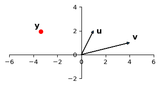
Consider a regression in which we are predicting the point \(\mathbf{y}\) as a linear function of two \(X\) columns, which we’ll denote \(\mathbf{u}\) and \(\mathbf{v}\).
Code
ax = ut.plotSetup(size=(4, 2))
ut.centerAxes(ax)
u = np.array([1, 2])
v = np.array([4, 1])
alph = 1.6
beta = -1.25
sum_uv = (alph * u) + (beta * v)
ax.arrow(0, 0, u[0], u[1], head_width=0.2, head_length=0.2, length_includes_head = True)
ax.arrow(0, 0, v[0], v[1], head_width=0.2, head_length=0.2, length_includes_head = True)
ax.arrow(0, 0, alph * u[0], alph * u[1], head_width=0.2,
         head_length=0.2, length_includes_head = True)
ax.arrow(alph * u[0], alph * u[1], sum_uv[0] - alph * u[0], sum_uv[1] - alph * u[1],
         head_width=0.2,
         head_length=0.2, length_includes_head = True, color = 'r')
ax.text(sum_uv[0]-2, sum_uv[1]+0.25, r'$\beta_1{\bf u}$+$\beta_2{\bf v}$',size=12)
ax.text(u[0]+0.25, u[1]-0.25, r'${\bf u}$', size=12)
ax.text(alph * u[0]+0.25, alph * u[1]-0.25, r'$\beta_1{\bf u}$', size=12)
ax.text(-2, 2.75, r'$\beta_2{\bf v}$', size=12)
ax.text(v[0]+0.25, v[1]+0.25, r'${\bf v}$',size=12)
ut.plotPoint(ax, sum_uv[0], sum_uv[1])
ax.plot(0, 0, '')
plt.show()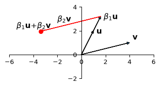
We determine the coefficients \(\beta_1\) and \(\beta_2\).
Now consider if the columns of \(X\) are nearly dependent.
Code
ax = ut.plotSetup(size=(4, 2))
ut.centerAxes(ax)
u = np.array([2, 1])
v = np.array([4, 1])
ax.arrow(0, 0, u[0], u[1], head_width=0.2, head_length=0.2, length_includes_head = True)
ax.arrow(0, 0, v[0], v[1], head_width=0.2, head_length=0.2, length_includes_head = True)
ax.text(sum_uv[0]-.5, sum_uv[1]+0.25, r'$\mathbf{y}$',size=12)
ax.text(u[0]+0.25, u[1]-0.25, r'${\bf u}$', size=12)
ax.text(v[0]+0.25, v[1]+0.25, r'${\bf v}$',size=12)
ut.plotPoint(ax, sum_uv[0], sum_uv[1])
ax.plot(0, 0, '')
plt.show()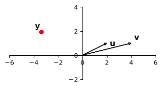
Code
ax = ut.plotSetup(size=(4, 2))
ut.centerAxes(ax)
u = np.array([2, 1])
v = np.array([4, 1])
alph = 2.675
beta = -8.75
ax.arrow(0, 0, u[0], u[1], head_width=0.2, head_length=0.2, length_includes_head = True)
ax.arrow(0, 0, v[0], v[1], head_width=0.2, head_length=0.2, length_includes_head = True)
ax.arrow(0, 0, alph * u[0], alph * u[1], head_width=0.2,
         head_length=0.2, length_includes_head = True)
ax.arrow(alph * u[0], alph * u[1], sum_uv[0] - alph * u[0], sum_uv[1] - alph * u[1],
         head_width=0.2,
         head_length=0.2, length_includes_head = True, color = 'r')
ax.text(sum_uv[0]-2, sum_uv[1]+0.25, r'$\beta_1{\bf u}$+$\beta_2{\bf v}$',size=12)
ax.text(u[0]+0.25, u[1]-0.25, r'${\bf u}$', size=12)
ax.text(alph * u[0]+0.25, alph * u[1]-0.25, r'$\beta_1{\bf u}$', size=12)
ax.text(-2, 2.75, r'$\beta_2{\bf v}$', size=12)
ax.text(v[0]+0.25, v[1]+0.25, r'${\bf v}$',size=12)
ut.plotPoint(ax, sum_uv[0], sum_uv[1])
ax.plot(0, 0, '')
plt.show()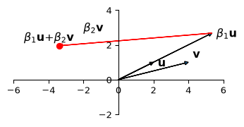
If you imagine the values of \(\beta_1\) and \(\beta_2\) necessary to create \(\mathbf{y} = \beta_1{\bf u}\)+\(\beta_2{\bf v}\), you can see that \(\beta_1\) and \(\beta_2\) will be very large in magnitude.
This geometric argument illustrates why the regression coefficients will be very large under multicollinearity.
As a result, the value of \(\Vert\boldsymbol{\beta}\Vert_2\) will be very large.
Ridge Regression
Ridge regression adjusts the least squares regression by shrinking the estimated coefficients towards zero.
The purpose is to fix the magnitude inflation of \(\Vert\boldsymbol{\beta}\Vert_2\).
To do this, Ridge regression assumes that the model has no intercept term – both the response and the predictors have been centered so that \(\beta_0 = 0\).
Ridge regression then consists of adding a penalty term to the regression:
\[ \hat{\boldsymbol{\beta}} = \arg \min_\boldsymbol{\beta} \Vert X\boldsymbol{\beta} - y \Vert_2^2 + c\Vert\boldsymbol{\beta}\Vert_2^2. \]
For any given \(c\) this has a closed-form solution in which \(\hat{\boldsymbol{\beta}} = (X^TX +cI)^{−1}X^T\mathbf{y}.\)
The solution to the Ridge regression problem always exists and is unique, even when the data contains multicollinearity.
Here, \(c \geq 0\) is a tradeoff parameter and controls the strength of the penalty term:
- When \(c = 0\), we get the least squares estimator: \(\hat{\boldsymbol{\beta}} = (X^TX)^{−1}X^T\mathbf{y}\)
- When \(c \rightarrow \infty\), we get \(\hat{\boldsymbol{\beta}} \rightarrow 0.\)
- Increasing the value of \(c\) forces the norm of \(\hat{\boldsymbol{\beta}}\) to decrease, yielding smaller coefficient estimates in magnitude.
For a finite, positive value of \(c\), we are balancing two tasks: fitting a linear model and shrinking the coefficients.
The coefficient \(c\) is a hyperparameter that controls the model complexity. We typically set \(c\) by holding out data, i.e., cross-validation.
Scaling
Note that the penalty term \(\Vert\boldsymbol{\beta}\Vert_2^2\) would be unfair to the different predictors if they are not on the same scale.
Therefore, if we know that the variables are not measured in the same units, we typically first perform unit normal scaling on the columns of \(X\) and on \(\mathbf{y}\) (to standardize the predictors), and then perform ridge regression.
Note that by scaling \(\mathbf{y}\) to have zero-mean, we do not need (or include) an intercept in the model.
Another name for ridge regression is Tikhanov regularization. You may see this terminology used in textbooks on optimization.
Normalizing is needed for this specific method. This is in contrast to the linear regression lecture where we allowed the coefficients to correct for the scaling differences between different units of measure.
Here is the performance of Ridge regression on the Longley data.
We are training on half of the data and using the other half for testing.
Code
from sklearn.metrics import r2_score
nreps = 1000

from sklearn.preprocessing import StandardScaler
scaler = StandardScaler()
X_std = scaler.fit_transform(X[['GNPDEFL', 'GNP', 'UNEMP', 'ARMED', 'POP']])
y_std = scaler.fit_transform(y.values.reshape(-1, 1))

np.random.seed(1)

vals = []
for alpha in np.r_[np.array([0]), 10**np.linspace(-8.5, -0.5, 20)]:
    res = []
    for rep in range(nreps):
        X_train, X_test, y_train, y_test = model_selection.train_test_split(
            X_std, y_std,
            test_size=0.5)
        model = sm.OLS(y_train, X_train)
        results = model.fit_regularized(alpha = alpha, L1_wt = 0)
        y_oos_predict = results.predict(X_test)
        r2_test = r2_score(y_test, y_oos_predict)
        res.append(r2_test)
    vals.append([alpha, np.mean(res), np.std(res)/np.sqrt(nreps)])

results = np.array(vals)
Code
ax = plt.figure(figsize = (6, 4)).add_subplot()
ax.errorbar(np.log10(results[1:][:, 0]), results[1:][:, 1],
            results[1:][:, 2],
            label = 'Ridge Regression')
ax.hlines(results[0,1], np.log10(results[1, 0]),
           np.log10(results[-1, 0]), linestyles = 'dashed',
          label = 'Without Regularization')
ax.hlines(results[0,1]+results[0,2], np.log10(results[1, 0]),
           np.log10(results[-1, 0]), linestyles = 'dotted')
ax.hlines(results[0,1]-results[0,2], np.log10(results[1, 0]),
           np.log10(results[-1, 0]), linestyles = 'dotted')
ax.tick_params(labelsize=12)
ax.set_ylabel('$R^2$', fontsize = 14)
plt.legend(loc = 'best')
ax.set_xlabel('$\\log_{10}(c)$', fontsize = 14)
ax.set_title('Ridge Regression Accuracy on Longley Data', fontsize = 16)
plt.show()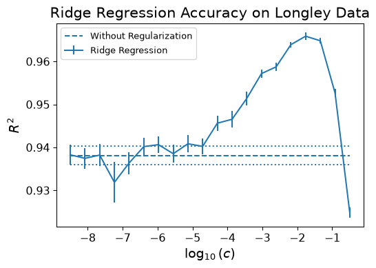
To sum up the idea behind Ridge regression:
- There may be many \(\boldsymbol{\beta}\) values that are consistent with the equations.
- Over-fit \(\boldsymbol{\beta}\) values tend to have large magnitudes.
- We add the regularization term \(c \Vert \boldsymbol{\beta}\Vert_2^2\) to the least squares to avoid those solutions.
- We tune \(c\) to an appropriate value via cross-validation.
Model Selection
Of course, one might attack the problem of multicollinearity as follows:
- Multicollinearity occurs when variables (features) are close to linearly dependent.
- These variables do not contribute anything meaningful to the quality of the model
- As a result why not simply remove variables from the model that are nearly linearly dependent?
We create a new model when we remove these variables from our regression.
This strategy is called model selection.
One of the advantages of model selection is interpretability: by eliminating variables, we get a clearer picture of the relationship between truly useful features and dependent variables.
However, there is a big challenge inherent in model selection. In general, the possibilities to consider are exponential in the number of features.
That is, if we have \(n\) features to consider, then there are \(2^n-1\) possible models that incorporate one or more of those features. This space is usually too big to search directly.
Can we use Ridge regression for this problem?
Ridge regression does not set any coefficients exactly to zero unless \(c\rightarrow \infty\), in which case they’re all zero.
This means Ridge regression cannot perform variable selection. Even though it performs well in terms of prediction accuracy, it does not offer a clear interpretation.
The LASSO
LASSO differs from Ridge regression only in terms of the norm used by the penalty term.
\[ \hat{\beta} = \arg \min_\beta \Vert X\beta - y \Vert_2^2 + c \Vert\beta\Vert_1. \]
However, this small change in the norm makes a big difference in practice.
The nature of the \(\ell_1\) penalty will cause some coefficients to be shrunken to zero exactly.
This means that LASSO can perform model selection by telling us which variables to keep and which to set aside.
As \(c\) increases, more coefficients are set to zero, i.e., fewer variables are selected.
In terms of prediction error, LASSO performs comparably to Ridge regression but it has a big advantage with respect to interpretation.
Code
from sklearn.metrics import r2_score
nreps = 200

from sklearn.preprocessing import StandardScaler
scaler = StandardScaler()
X_std = scaler.fit_transform(X[['GNPDEFL', 'GNP', 'UNEMP', 'ARMED', 'POP']])
X_std = np.column_stack([X_std, np.ones(X_std.shape[0])])
y_std = scaler.fit_transform(y.values.reshape(-1, 1))

np.random.seed(1)

vals = []
mean_params = []
for alpha in np.r_[np.array([0]), 10**np.linspace(-5, -0.75, 10)]:
    res = []
    params = []
    for rep in range(nreps):
        X_train, X_test, y_train, y_test = model_selection.train_test_split(
            X_std, y_std,
            test_size=0.5)
        model = sm.OLS(y_train, X_train)
        results = model.fit_regularized(alpha = alpha, L1_wt = 1.0)
        y_oos_predict = results.predict(X_test)
        r2_test = r2_score(y_test, y_oos_predict)
        res.append(r2_test)
        params.append(results.params)
    vals.append([alpha, np.mean(res), np.std(res)/np.sqrt(nreps)])
    mean_params.append(np.r_[alpha, np.mean(params, axis = 0)])
results = np.array(vals)
mean_params = np.array(mean_params)
Code
ax = plt.figure(figsize = (6, 4)).add_subplot()
ax.errorbar(np.log10(results[1:][:, 0]), results[1:][:, 1],
            results[1:][:, 2],
            label = 'LASSO Regression')
ax.hlines(results[0,1], np.log10(results[1, 0]),
           np.log10(results[-1, 0]), linestyles = 'dashed',
          label = 'Without Regularization')
ax.hlines(results[0,1]+results[0,2], np.log10(results[1, 0]),
           np.log10(results[-1, 0]), linestyles = 'dotted')
ax.hlines(results[0,1]-results[0,2], np.log10(results[1, 0]),
           np.log10(results[-1, 0]), linestyles = 'dotted')
ax.tick_params(labelsize=12)
ax.set_ylabel('$R^2$', fontsize = 14)
#ax.set_xlim([-4, -1])
plt.legend(loc = 'best')
ax.set_xlabel('$\\log_{10}(c)$', fontsize = 14)
ax.set_title('LASSO Accuracy on Longley Data', fontsize = 16)
plt.show()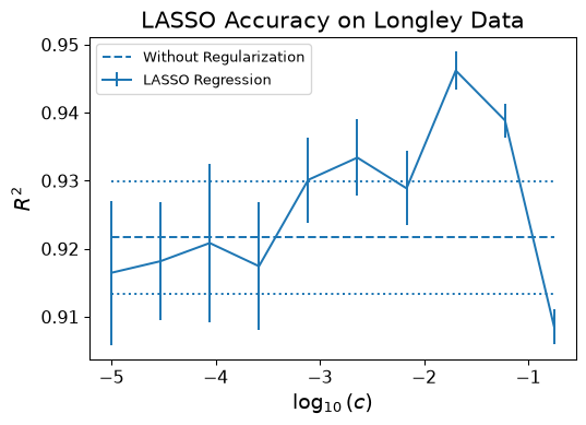
Code
df = pd.DataFrame(mean_params, columns = ['$\log_{10}(c)$', 'GNPDEFL', 'GNP', 'UNEMP', 'ARMED', 'POP', 'const'])
param_df = df[['GNPDEFL', 'GNP', 'UNEMP', 'ARMED', 'POP', 'const']].iloc[1:].copy()
param_df.index = np.log10(df.iloc[1:]['$\log_{10}(c)$'])
Code
param_df.plot()
plt.legend(loc='center left', bbox_to_anchor=(1, 0.5), prop={'size': 16})
plt.title('LASSO Coefficients vs $c$')
plt.show()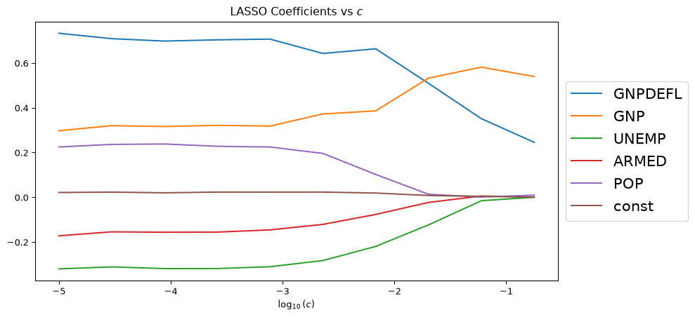
We can use the statsmodel smf sub-module to directly type formulas and expressions in the functions of the models. This allows us to, among other things,
- specify the name of the columns to be used to predict another column
- remove columns
- infer the type of the variable (e.g., categorical, numerical)
- apply functions to columns
The smf submodule makes use of the patsy package. patsy is a Python package for describing statistical models (especially linear models, or models that have a linear component) and building design matrices. It is closely inspired by and compatible with the formula mini-language used in R and S.
In the following code cells we will see the syntax that is used to specify columns in the models and how to remove columns from our model
Here is an example where we specify the name of the columns to be used to predict another column.
Code
X['TOTEMP'] = yCode
mod = smf.ols(formula='TOTEMP ~ GNPDEFL + GNP + UNEMP + ARMED + POP', data=X)
res = mod.fit()
with warnings.catch_warnings():
    warnings.simplefilter('ignore')
    print(res.summary())
OLS Regression Results
==============================================================================
Dep. Variable: TOTEMP R-squared: 0.987
Model: OLS Adj. R-squared: 0.981
Method: Least Squares F-statistic: 156.4
Date: Mon, 17 Aug 2026 Prob (F-statistic): 3.70e-09
Time: 17:09:59 Log-Likelihood: -117.83
No. Observations: 16 AIC: 247.7
Df Residuals: 10 BIC: 252.3
Df Model: 5
Covariance Type: nonrobust
==============================================================================
coef std err t P>|t| [0.025 0.975]
------------------------------------------------------------------------------
Intercept 9.246e+04 3.52e+04 2.629 0.025 1.41e+04 1.71e+05
GNPDEFL -48.4628 132.248 -0.366 0.722 -343.129 246.204
GNP 0.0720 0.032 2.269 0.047 0.001 0.143
UNEMP -0.4039 0.439 -0.921 0.379 -1.381 0.573
ARMED -0.5605 0.284 -1.975 0.077 -1.193 0.072
POP -0.4035 0.330 -1.222 0.250 -1.139 0.332
==============================================================================
Omnibus: 1.572 Durbin-Watson: 1.248
Prob(Omnibus): 0.456 Jarque-Bera (JB): 0.642
Skew: 0.489 Prob(JB): 0.725
Kurtosis: 3.079 Cond. No. 1.21e+08
==============================================================================
Notes:
[1] Standard Errors assume that the covariance matrix of the errors is correctly specified.
[2] The condition number is large, 1.21e+08. This might indicate that there are
strong multicollinearity or other numerical problems.The formula
formula='TOTEMP ~ GNPDEFL + GNP + UNEMP + ARMED + POP'
is an R-style formula string that specifies the model.
The variable TOTEMP is the dependent variable, which is Total Employment in the Longley dataset.
The syntax ~ separates the dependent variable from the independent variables.
The sytnax GNPDEFL + GNP + UNEMP + ARMED + POP are the independent variables, which are GNP Deflator, Gross National Product, Number of Unemployed, Size of the Armed Forces, and Population.
This is an example where we remove columns from the data and exclude the y-intercept.
Code
mod = smf.ols(formula='TOTEMP ~ GNPDEFL + GNP + UNEMP - 1', data=X)
res = mod.fit()
with warnings.catch_warnings():
    warnings.simplefilter('ignore')
    print(res.summary())
OLS Regression Results
=======================================================================================
Dep. Variable: TOTEMP R-squared (uncentered): 1.000
Model: OLS Adj. R-squared (uncentered): 1.000
Method: Least Squares F-statistic: 1.127e+04
Date: Mon, 17 Aug 2026 Prob (F-statistic): 1.92e-22
Time: 17:09:59 Log-Likelihood: -137.20
No. Observations: 16 AIC: 280.4
Df Residuals: 13 BIC: 282.7
Df Model: 3
Covariance Type: nonrobust
==============================================================================
coef std err t P>|t| [0.025 0.975]
------------------------------------------------------------------------------
GNPDEFL 871.0961 25.984 33.525 0.000 814.961 927.231
GNP -0.0532 0.007 -8.139 0.000 -0.067 -0.039
UNEMP -0.8333 0.496 -1.679 0.117 -1.905 0.239
==============================================================================
Omnibus: 0.046 Durbin-Watson: 1.422
Prob(Omnibus): 0.977 Jarque-Bera (JB): 0.274
Skew: -0.010 Prob(JB): 0.872
Kurtosis: 2.359 Cond. No. 2.92e+04
==============================================================================
Notes:
[1] R² is computed without centering (uncentered) since the model does not contain a constant.
[2] Standard Errors assume that the covariance matrix of the errors is correctly specified.
[3] The condition number is large, 2.92e+04. This might indicate that there are
strong multicollinearity or other numerical problems.The formula is
formula='TOTEMP ~ GNPDEFL + GNP + UNEMP - 1'
We still have the same dependent variable TOTEMP. The independent variables are GNPDEFL + GNP + UNEMP
The syntax -1 removes the intercept from the model. By default, an intercept is included in the model, but - 1 explicitly excludes it.
The LASSO and Longley Data
Here are some of the important observations from using LASSO regression on the Longley dataset:
- We removed the near linearly dependent features from our model.
- We improved the condition number of the data by 4 orders of magnitude.
- There is only one variable whose condfidence interval contains 0.
Flexible Modeling
To look at model selection in practice, we will consider another famous dataset.
The Guerry dataset is a collection of historical data used in support of Andre-Michel Guerry’s 1833 “Essay on the Moral Statistics of France.”
Andre-Michel Guerry’s (1833) Essai sur la Statistique Morale de la France was one of the foundation studies of modern social science. Guerry assembled data on crimes, suicides, literacy and other “moral statistics,” and used tables and maps to analyze a variety of social issues in perhaps the first comprehensive study relating such variables.
Guerry’s results were startling for two reasons. First he showed that rates of crime and suicide remained remarkably stable over time, when broken down by age, sex, region of France and even season of the year; yet these numbers varied systematically across departements of France. This regularity of social numbers created the possibility to conceive, for the first time, that human actions in the social world were governed by social laws, just as inanimate objects were governed by laws of the physical world.
Source: “A.-M. Guerry’s Moral Statistics of France: Challenges for Multivariable Spatial Analysis”, Michael Friendly. Statistical Science 2007, Vol. 22, No. 3, 368–399.
Here is the dataset.
Code
# Lottery is per-capital wager on Royal Lottery
df = sm.datasets.get_rdataset("Guerry", "HistData").data
df = df[['Lottery', 'Literacy', 'Wealth', 'Region']].dropna()
df.head()| Lottery | Literacy | Wealth | Region | |
|---|---|---|---|---|
| 0 | 41 | 37 | 73 | E |
| 1 | 38 | 51 | 22 | N |
| 2 | 66 | 13 | 61 | C |
| 3 | 80 | 46 | 76 | E |
| 4 | 79 | 69 | 83 | E |
Here is a regression using the feature Literacy, Wealth, and Region.
Code
mod = smf.ols(formula='Lottery ~ Literacy + Wealth + Region', data=df)
res = mod.fit()
print(res.summary())
OLS Regression Results
==============================================================================
Dep. Variable: Lottery R-squared: 0.338
Model: OLS Adj. R-squared: 0.287
Method: Least Squares F-statistic: 6.636
Date: Mon, 17 Aug 2026 Prob (F-statistic): 1.07e-05
Time: 17:10:00 Log-Likelihood: -375.30
No. Observations: 85 AIC: 764.6
Df Residuals: 78 BIC: 781.7
Df Model: 6
Covariance Type: nonrobust
===============================================================================
coef std err t P>|t| [0.025 0.975]
-------------------------------------------------------------------------------
Intercept 38.6517 9.456 4.087 0.000 19.826 57.478
Region[T.E] -15.4278 9.727 -1.586 0.117 -34.793 3.938
Region[T.N] -10.0170 9.260 -1.082 0.283 -28.453 8.419
Region[T.S] -4.5483 7.279 -0.625 0.534 -19.039 9.943
Region[T.W] -10.0913 7.196 -1.402 0.165 -24.418 4.235
Literacy -0.1858 0.210 -0.886 0.378 -0.603 0.232
Wealth 0.4515 0.103 4.390 0.000 0.247 0.656
==============================================================================
Omnibus: 3.049 Durbin-Watson: 1.785
Prob(Omnibus): 0.218 Jarque-Bera (JB): 2.694
Skew: -0.340 Prob(JB): 0.260
Kurtosis: 2.454 Cond. No. 371.
==============================================================================
Notes:
[1] Standard Errors assume that the covariance matrix of the errors is correctly specified.In the previous cell, using the patsy syntax determined that elements of Region were text strings, so it treated Region as a categorical variable.
Alternatively, we could manually enforce this with the syntax on the following slide. Recall that the - sign is used to remove columns/variables. Here we remove the intercept from a model by.
Code
res = smf.ols(formula='Lottery ~ Literacy + Wealth + C(Region) -1 ', data=df).fit()
print(res.summary())
OLS Regression Results
==============================================================================
Dep. Variable: Lottery R-squared: 0.338
Model: OLS Adj. R-squared: 0.287
Method: Least Squares F-statistic: 6.636
Date: Mon, 17 Aug 2026 Prob (F-statistic): 1.07e-05
Time: 17:10:00 Log-Likelihood: -375.30
No. Observations: 85 AIC: 764.6
Df Residuals: 78 BIC: 781.7
Df Model: 6
Covariance Type: nonrobust
================================================================================
coef std err t P>|t| [0.025 0.975]
--------------------------------------------------------------------------------
C(Region)[C] 38.6517 9.456 4.087 0.000 19.826 57.478
C(Region)[E] 23.2239 14.931 1.555 0.124 -6.501 52.949
C(Region)[N] 28.6347 13.127 2.181 0.032 2.501 54.769
C(Region)[S] 34.1034 10.370 3.289 0.002 13.459 54.748
C(Region)[W] 28.5604 10.018 2.851 0.006 8.616 48.505
Literacy -0.1858 0.210 -0.886 0.378 -0.603 0.232
Wealth 0.4515 0.103 4.390 0.000 0.247 0.656
==============================================================================
Omnibus: 3.049 Durbin-Watson: 1.785
Prob(Omnibus): 0.218 Jarque-Bera (JB): 2.694
Skew: -0.340 Prob(JB): 0.260
Kurtosis: 2.454 Cond. No. 653.
==============================================================================
Notes:
[1] Standard Errors assume that the covariance matrix of the errors is correctly specified.We can also apply vectorized functions to the variables in our model. The following cell shows how to do this. In this case we apply the natural log function to the Literacy column and use this single column to predict the Lottery values.
Code
res = smf.ols(formula='Lottery ~ np.log(Literacy)', data=df).fit()
print(res.summary())
OLS Regression Results
==============================================================================
Dep. Variable: Lottery R-squared: 0.161
Model: OLS Adj. R-squared: 0.151
Method: Least Squares F-statistic: 15.89
Date: Mon, 17 Aug 2026 Prob (F-statistic): 0.000144
Time: 17:10:00 Log-Likelihood: -385.38
No. Observations: 85 AIC: 774.8
Df Residuals: 83 BIC: 779.7
Df Model: 1
Covariance Type: nonrobust
====================================================================================
coef std err t P>|t| [0.025 0.975]
------------------------------------------------------------------------------------
Intercept 115.6091 18.374 6.292 0.000 79.064 152.155
np.log(Literacy) -20.3940 5.116 -3.986 0.000 -30.570 -10.218
==============================================================================
Omnibus: 8.907 Durbin-Watson: 2.019
Prob(Omnibus): 0.012 Jarque-Bera (JB): 3.299
Skew: 0.108 Prob(JB): 0.192
Kurtosis: 2.059 Cond. No. 28.7
==============================================================================
Notes:
[1] Standard Errors assume that the covariance matrix of the errors is correctly specified.Recap
We discussed how to perform regularization in linear regression to avoid issues of overfitting due to multicollinearity.
We discussed how the condition number of a matrix indicates whether we have issues with multicollinearity.
We saw that large condition numbers indicate multicollinearity.
To address this issue we considered both Ridge and LASSO regression.
We also learned about the patsy syntax in the statsmodel package.