Recap: Linear Regression
DS701 Session 12 — Wed Oct 14, 2026


Today’s plan
- 5 min — knowledge-check review
- 20 min — highlights and Q&A (answer or pass — answering always earns credit)
- 45 min — case study: predicting diabetes progression
- wrap-up and cold-call check-ins
Knowledge-Check Review
KC 1: The objective and the equations
In one or two sentences: what does the least-squares line minimize, and what are the normal equations that its coefficients \(\hat\beta\) satisfy? (Write the equations; no derivation needed.)
Show answer
Answer. It minimizes the sum of squared residuals
\[ \sum_i \bigl(y_i - \beta_0 - \beta_1 x_i\bigr)^2 = \lVert X\beta - \mathbf{y}\rVert^2 , \]
the squared distance between the predictions \(X\beta\) and the observations \(\mathbf{y}\). The minimizer solves the normal equations
\[ X^\top X\,\beta = X^\top \mathbf{y}, \qquad \hat\beta = (X^\top X)^{-1}X^\top\mathbf{y} \ \text{ when } X^\top X \text{ is invertible.} \]
KC 2: Why \(R^2\) only ever goes up
\(R^2 = 1 - \text{RSS}/\text{TSS}\) is “the fraction of the variance of \(y\) explained by the model.” Explain why \(R^2\) can never go down when you add another feature (column) to \(X\) and refit — and why that makes a high in-sample \(R^2\) weak evidence on its own that the model is good.
Show answer
Answer. A new column enlarges the column space of \(X\). The old fit is still available (give the new column coefficient \(0\)), so the least-squares minimum of RSS over the bigger space can only be as low or lower — RSS cannot rise, so \(R^2\) cannot fall.
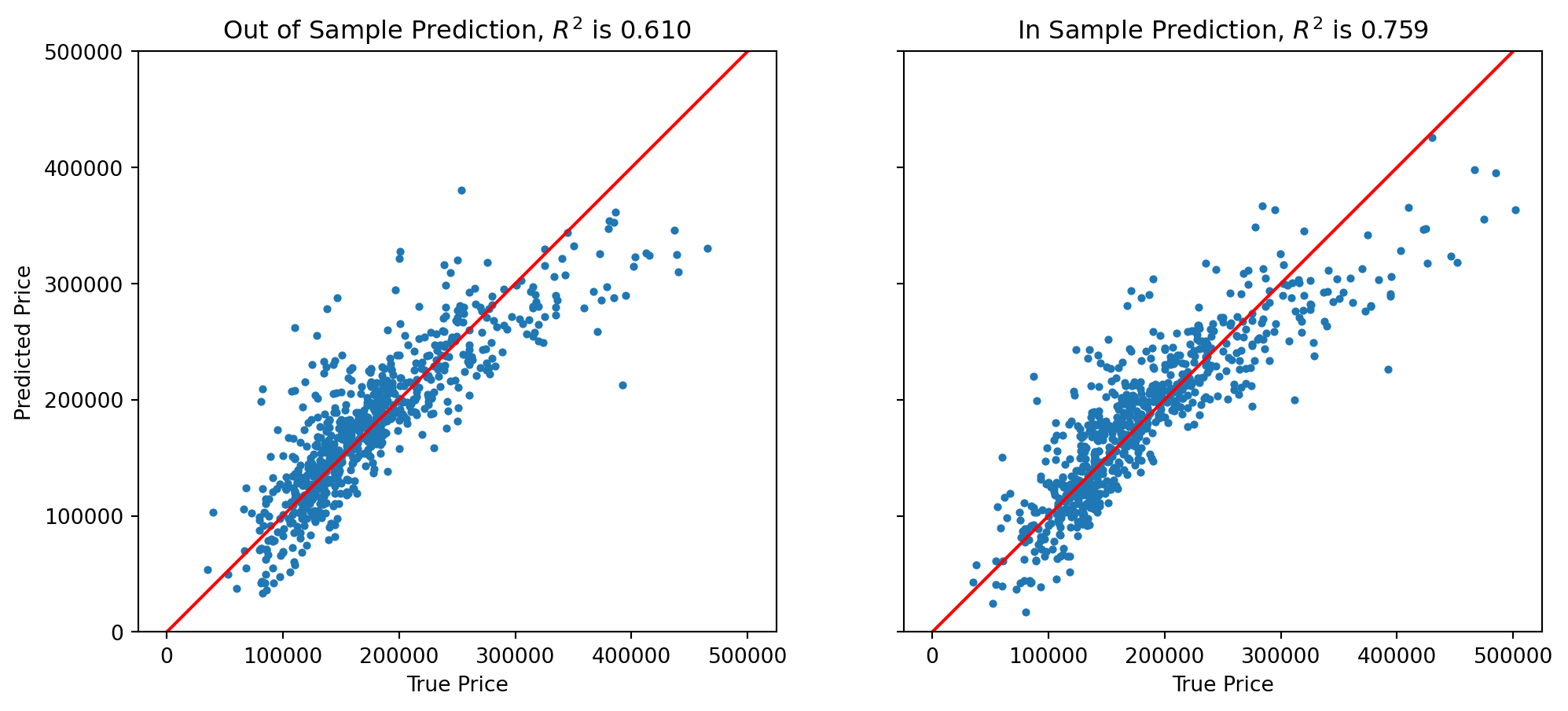
Hence even a random column nudges \(R^2\) up: in-sample \(R^2\) rewards fitting, noise included. That is why the lecture judged the Ames model on held-out houses (0.61 out-of-sample vs 0.76 in-sample), and why the summary reports adjusted \(R^2\) and confidence intervals alongside it.
KC 3: “Linear” means linear in \(\beta\)
A colleague says “linear regression can only fit straight lines, so it is useless for my data, which clearly curves.” Using the lecture’s fits of a parabola and of \(y = \beta_0 + \beta_1 \log x\), explain what “linear” in linear model* actually refers to, and what changes (and what does not) in the least-squares procedure when you fit a curve.*
Show answer
Answer. Linear in the parameters: any \(y = \beta_0 f_0(x) + \beta_1 f_1(x) + \cdots\) with known \(f_j\) is a linear model. Parabola: \(X = [\mathbf{1},\ x,\ x^2]\). Log model: \(X = [\mathbf{1},\ \log x]\).
Nothing else changes — same normal equations, same \(\hat\beta = (X^\top X)^{-1}X^\top\mathbf{y}\), same \(R^2\). What is not linear: \(y = \beta_0 e^{-\beta_1 x}\) — a parameter inside a nonlinear function.
Highlights
The model, the residual, the objective
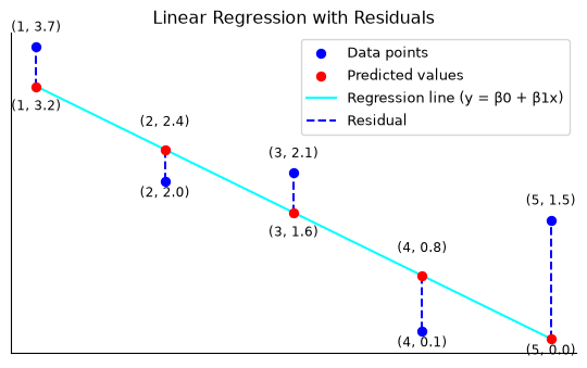
- Model: \(y = \beta_0 + \beta_1 x + \epsilon\) — a line plus a residual.
- Stack the \(n\) equations: \(\mathbf{y} = X\beta + \boldsymbol\epsilon\), with \(X = [\mathbf{1},\ \mathbf{x}]\) the design matrix.
- No \(\beta\) makes \(X\beta = \mathbf{y}\) exactly — so we ask for the \(\beta\) that makes them closest: \[\min_\beta \ \sum_i \epsilon_i^2 = \min_\beta \ \lVert X\beta - \mathbf{y}\rVert^2 .\]
- The sum of squared residuals is a squared distance. That single sentence is why linear algebra solves regression.
Least squares is a projection
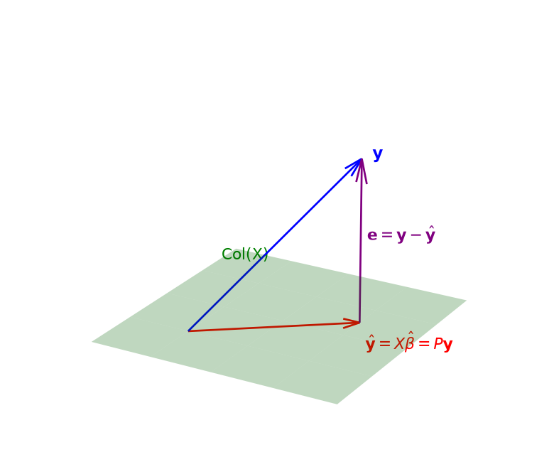
- \(X\beta\) ranges over the column space of \(X\). The closest point to \(\mathbf{y}\) in that space is its orthogonal projection \(\hat{\mathbf{y}}\).
- So the residual \(\mathbf{e} = \mathbf{y} - X\hat\beta\) is perpendicular to every column of \(X\): \[X^\top(\mathbf{y} - X\hat\beta) = \mathbf{0} \;\Longleftrightarrow\; X^\top X\hat\beta = X^\top\mathbf{y}.\] That is where the normal equations come from.
- Substituting: \(\hat{\mathbf{y}} = X(X^\top X)^{-1}X^\top\mathbf{y} = P\mathbf{y}\) — the projection (hat) matrix, symmetric, \(P^2 = P\), trace \(= p\).
- Two consequences you will verify today: residuals sum to zero (the \(\mathbf{1}\) column), and \(\text{TSS} = \text{RSS} + \text{ESS}\) (Pythagoras in \(\mathbb{R}^n\)).
Same equations, any design matrix
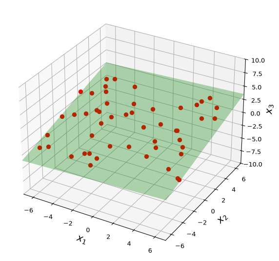
Once \(X\) is built, the procedure never changes:
| model | columns of \(X\) |
|---|---|
| line | \(\mathbf{1},\ x\) |
| parabola | \(\mathbf{1},\ x,\ x^2\) |
| log | \(\mathbf{1},\ \log x\) |
| plane / multiple regression | \(\mathbf{1},\ u,\ v,\ \dots\) |
| trend surface | \(\mathbf{1},\ u,\ v,\ u^2,\ uv,\ v^2\) |
“Linear” = linear in \(\beta\). Requirements for a unique \(\hat\beta\): full column rank (\(n \ge p\), no column a combination of the others) — otherwise \(X^\top X\) is singular and the coefficients, though not the fit, are undetermined.
Reading the answer: coefficients
From the Ames model (seven features, sale price in dollars):
| feature | \(\hat\beta\) | reads as |
|---|---|---|
| gross living area | $48 / sq ft | one more square foot, other features held fixed |
| full bath | $14,900 | one more full bath, others fixed |
| garage area | $99 / sq ft | |
| lot area | $0.23 / sq ft | CI includes 0 — not distinguishable from no effect |
- Units live in \(\beta\): no feature scaling needed (unlike \(k\)-means / \(k\)-NN).
- A coefficient is a conditional slope.
- estimated change in the target variable (\(y\)) for a one-unit change in a specific feature (\(x_i\)), holding all other features constant.
- Add a correlated feature and the others move — you will watch that happen today.
- A CI that covers zero says the data cannot tell that coefficient from zero. The lecture dropped such columns – with a warning that selecting features and scoring the refit on the same data flatters it.
- None of this is a causal claim (Session 18 is about why).
Reading the answer: \(R^2\) — and its limits
\[R^2 = \frac{\text{ESS}}{\text{TSS}} = 1 - \frac{\text{RSS}}{\text{TSS}} \in [0, 1]\]
- Fraction of the variance of \(y\) the model explains. Not Pearson’s \(r\).
- Never decreases when a column is added → in-sample \(R^2\) cannot choose between models.
- Honest number: \(R^2\) on held-out data (0.61 vs 0.76 here).
- And look at the picture: predictions bend away from the diagonal at both ends — \(\text{Var}(\hat{\mathbf y}) \le \text{Var}(\mathbf y)\), Galton’s regression to the mean out of the algebra. \(R^2\) did not tell you that — the residuals did.
The diagnostic habit: plot the residuals
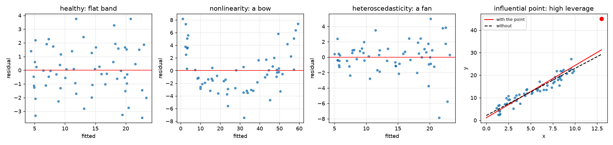
- \(\hat\beta\) and \(R^2\) are computed assuming the model. Only the residuals test the assumption.
- Residuals vs fitted should be a flat, even band. A bow = a missing term (nonlinearity). A fan = spread grows with the fit (heteroscedasticity). One point far out in \(x\) = high leverage — it can tilt the whole line and fake the other two patterns.
- Leverage is \(P_{ii}\), the diagonal of today’s projection matrix — the linear algebra and the diagnostics are the same object.
- The lecture’s Ames residual plot shows two of these at once: a fan, and two 4,000+ sq ft houses the model prices at $550k and $850k that sold for far less.
- Today’s Part 4: run these diagnostics on the care-management program’s model and answer their question — does it fit all patients equally?
Going deeper
Full lecture notes: Linear Regression
- Least-Squares Lines — residuals and the objective
- A least-squares problem — \(X\beta = \mathbf{y}\) and the objective
- Least squares is a projection and The hat matrix — where the normal equations come from; when \(X^\top X\) is invertible
- Least-Squares Fitting of Other Models — parabola and log fits; linear in \(\beta\)
- Multiple Regression — the least-squares plane
- Measuring the fit: \(R^2\) and TSS = RSS + ESS — the orthogonality behind the identity
- Aside: Summary Statistics — reading a statsmodels table
- House Prices in Ames, Iowa — coefficients in dollars as conditional slopes, in- vs out-of-sample \(R^2\), and the residuals-vs-fitted plot
- Next lecture: when \(y\) is a category (logistic regression), and when \(\beta\) overfits (regularization)
In-Class Activity
Activity — Case Study 10: Diabetes Progression
The client: a primary-care network’s diabetes care-management program.
- Which baseline measurements predict disease progression a year later?
- Can nurses use the model to prioritize outreach?
- Can the model’s numbers be trusted?
The data: the public scikit-learn diabetes study
- 200 patients — your section’s subset
- A prototype until the network’s own records are released
Activity — The Four Parts
- Fit: build \(X\) with an intercept, solve the normal equations, check against
lstsqand scikit-learn, compute \(R^2\) - Project: form the projection matrix; check the residual is orthogonal to the columns
- Collinearity: add serum triglycerides (correlated) and watch the BMI coefficient move
- Diagnose: write a
diagnosticsfunction — does the model fit all patients equally?
Report out: the two sentences at the top of your memo to the program.
Activity — Logistics
- Work in groups of 2–3. Open your section’s notebook.
- Parts marked (autograded) are submitted to Gradescope; the rest is participation.
- Staff will circulate — be ready to explain any part of your work.
- Dependencies:
numpy,pandas,matplotlib,scipy,scikit-learn.


The activity notebook goes live on the day of the lecture. Colab is optional — you can also open it on GitHub and run it locally.