Recap: Neural Networks I — How Learning Works
DS701 Session 19 — Mon Nov 9, 2026


Today’s plan
- 5 min — knowledge-check review
- 20 min — highlights and Q&A (answer or pass — answering always earns credit)
- 45 min — case study: the model stopped learning after the refactor
- wrap-up and cold-call check-ins
- Final team project is assigned today — spec and team sign-up on Piazza after class.
Backprop by hand — the recipe from this lecture — is examined on Quiz 3; HW9 will practise it. Today’s activity is the first rep.
Knowledge-Check Review
KC 1: The recipe
State the backpropagation recipe from the lecture: what runs first and why, what the output node’s gradient is set to, and what each of the three node types (+, *, ReLU) does with the gradient that arrives from its parent.
KC 2: The chain rule by hand
Take the lecture’s three-stage graph, \(d = a \cdot b\), \(e = d + c\), \(L = e \cdot f\), but with new values \(a = 2\), \(b = -1\), \(c = 5\), \(f = 3\). Run the forward pass, then propagate backwards to find \(\partial L/\partial c\) and \(\partial L/\partial b\). Show the chain of local derivatives you multiplied for \(\partial L/\partial b\).
KC 3: Why gradient descent, and why mini-batches
In lecture 10 we solved linear regression in closed form (the normal equations). An MLP with an MSE loss also has a formula for its loss — so why do we train it by gradient descent instead of solving for the weights, and once we have chosen gradient descent, why do we compute the gradient on a mini-batch rather than on the whole training set every step?
Highlights
A neuron, a layer, a network — one composed function
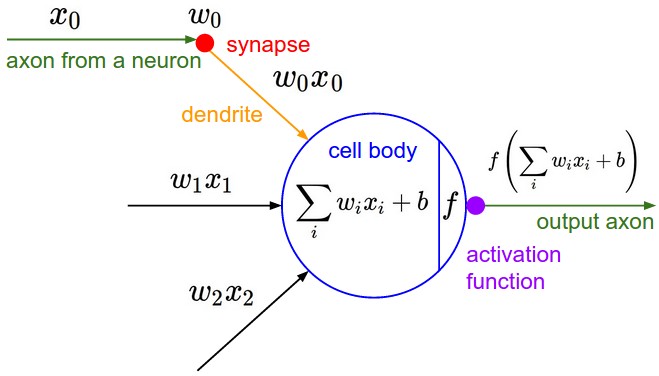
\[\text{out} = f\Big(\sum_i w_i x_i + b\Big)\]
- With \(f = \sigma\) this is logistic regression — weights, bias, squash.
- A layer: many neurons in parallel on the same inputs → \(\mathbf{h} = f(\boldsymbol\beta + \boldsymbol\Omega\mathbf{x})\).
- A network: layers in sequence, each layer’s outputs the next one’s inputs: \[\hat{\mathbf y} = \boldsymbol\beta_K + \boldsymbol\Omega_K\, f(\cdots f(\boldsymbol\beta_0 + \boldsymbol\Omega_0\mathbf{x})\cdots)\]
- So an MLP is a function of its parameters \(\theta = \{\boldsymbol\Omega_k, \boldsymbol\beta_k\}\) — and the activation \(f\) is what stops the stack collapsing to one linear map.
Training is a loop: loss → gradient → update
- Loss — a number that says how wrong the network is on the data: MSE \(\frac1N\sum(\hat y_i - y_i)^2\), or cross-entropy for classes.
- Gradient — \(\nabla_\theta L\): how the loss changes with every parameter.
- Update — step downhill: \[\theta \leftarrow \theta - \eta\,\nabla_\theta L\]
- Repeat until the loss stops falling.
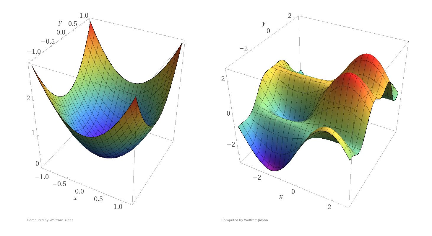
Non-convex surface: no closed form — you walk.
The learning rate decides: walk down or bounce out
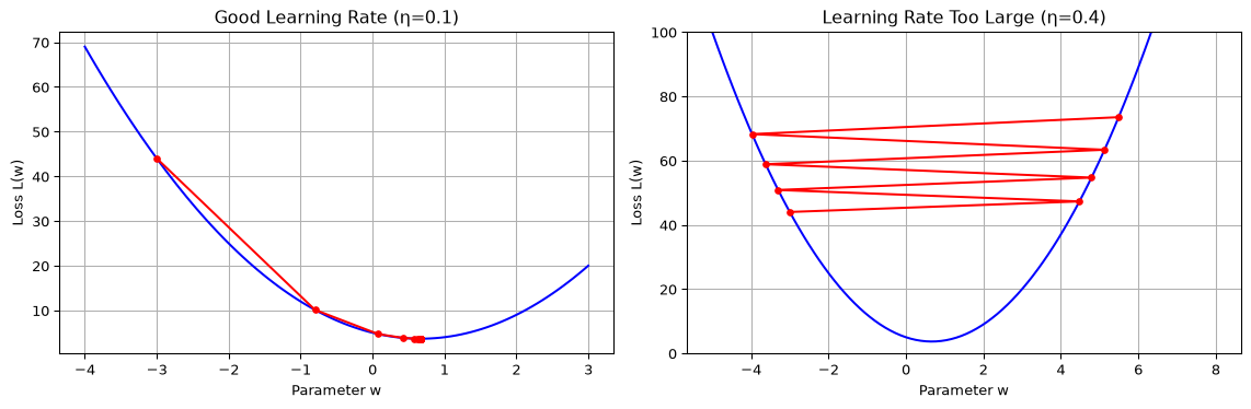
On \(L(w) = 3w^2 - 4w + 5\) each step multiplies the distance to the minimum by \((1 - 6\eta)\): \(\eta = 0.1\) gives \(0.4\) (converges), \(\eta = 1/3\) gives \(-1\) (bounces forever), \(\eta = 0.35\) gives \(-1.1\) (diverges).
Where do the gradients come from?
\[ L = \ell\big(\,\boldsymbol\beta_K + \boldsymbol\Omega_K\, f(\boldsymbol\beta_{K-1} + \boldsymbol\Omega_{K-1}\, f(\cdots f(\boldsymbol\beta_0 + \boldsymbol\Omega_0 \mathbf{x})\cdots)),\ y\big) \]
- By hand, for millions of parameters — hopeless.
- Numerically, wiggling each parameter — one or two forward passes per parameter.
- We want all the partials for a small multiple of the cost of one forward pass.
Backpropagation = the chain rule, organised on a computation graph. Record every operation as a node; store data (forward) and grad (backward) on each.

\(d = a\cdot b,\ e = d + c,\ L = e\cdot f\) — after the forward pass, every grad is still 0.
The chain rule, node by node
\[ \frac{\partial L}{\partial c} = \frac{\partial L}{\partial e}\cdot\frac{\partial e}{\partial c} \qquad\text{— gradient from above} \times \text{local derivative, both at the forward-pass values.} \]
L.grad = 1. Then \(L = e\cdot f\): \(\ \partial L/\partial e = f = 2,\ \ \partial L/\partial f = e = -4\) — a product hands each operand the other’s value.- \(e = d + c\): local derivative 1 — a sum just routes the gradient:
d.grad = c.grad = 2. - \(d = a\cdot b\):
b.grad = a.data * d.grad = 8,a.grad = b.data * d.grad = -6.

Check: wiggle \(b\) by 1 → \(L\) changes by 8. Every step was local — that is why it costs a small multiple of one forward pass, however many parameters.
The recipe on a real neuron

\(o = \mathrm{ReLU}(x_1w_1 + x_2w_2 + b)\), with \(x_1 = 2,\ x_2 = 0\).
o.grad = 1- ReLU: input was \(> 0\) →
n.grad = 1 - two
+nodes route it →x1w1.grad = x2w2.grad = b.grad = 1 *nodes:w1.grad = x1 · 1 = 2,w2.grad = x2 · 1 = 0
Then one step for each parameter leaf: \(w \leftarrow w - \eta\,\partial L/\partial w\).
Put a loss on top
\(z_1 = w_1x + b_1,\ h = \mathrm{ReLU}(z_1),\ \hat y = w_2h + b_2,\ L = \tfrac12(\hat y - y)^2\), with \(w_1 = 1,\ b_1 = 0.5,\ w_2 = -2,\ b_2 = 1\), one example \(x = 1,\ y = 0\).
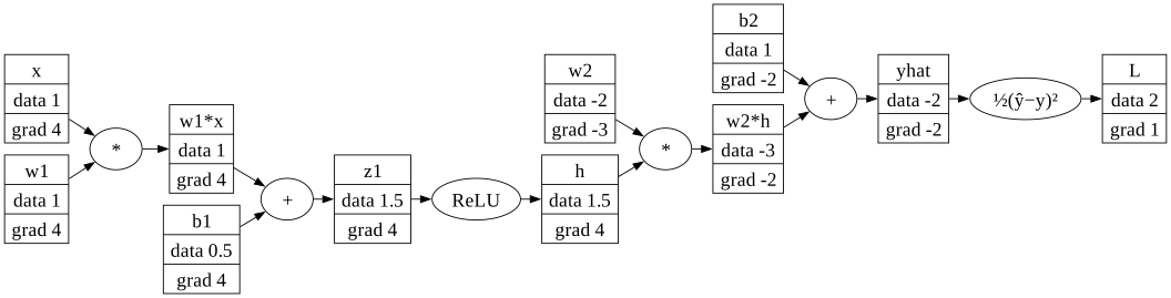
- Forward: \(z_1 = 1.5,\ h = 1.5,\ \hat y = -2,\ L = 2\). The loss node sends \(\hat y - y = -2\).
- Chain to \(w_1\): \((\hat y - y)\cdot w_2 \cdot \mathrm{ReLU}'(z_1)\cdot x = (-2)(-2)(1)(1) = 4\).
- One step, \(\eta = 0.05\): \(\hat y \to -0.935\), \(L: 2 \to 0.437\).
…and watch a ReLU die
Same parameters, input flipped to \(x = -1\): \(z_1 = -0.5 < 0\), so \(h = 0\), \(\hat y = 1\), \(L = \tfrac12\).
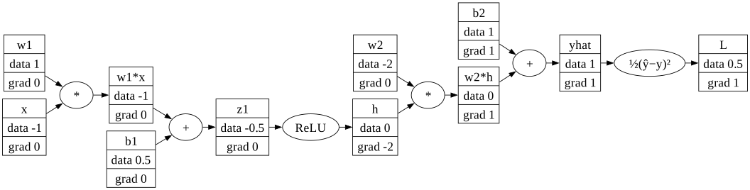
- \(\partial L/\partial w_2 = 0\) — the
*rule (its input \(h\) is 0). - \(\partial L/\partial w_1 = \partial L/\partial b_1 = 0\) — the closed ReLU gate zeroes everything upstream, although \(\partial L/\partial h = -2\). Only \(b_2\) learns: a dead ReLU.
The recipe, once more: forward pass; L.grad = 1; walk back multiplying by local derivatives — + routes, * swaps, ReLU gates, the loss node \(\tfrac12(\hat y - y)^2\) sends \(\hat y - y\). That is what you will implement, check against finite differences, and be asked to do on paper.
Why stochastic gradient descent
Backprop gives \(\nabla_\mathbf{w}\ell_i\) for one sample. How many before a step?
| per step | gradient | noise | |
|---|---|---|---|
| full batch | all \(N\) | exact | none |
| SGD (\(B=1\)) | 1 | very noisy | lots |
| mini-batch | \(B \approx 32\)–\(256\) | good enough | some |
Per unit of computation, mini-batch wins; on a non-convex surface its noise may also shake you out of a poor minimum (observed, not a theorem).
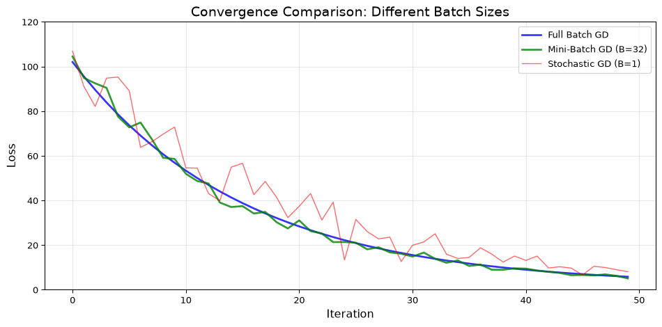
Real run (linear regression). Left: equal steps. Right: equal computation.
In-Class Activity
Activity — Case Study 16: The Model Stopped Learning After the Refactor
Goal: you have just joined an ML platform team whose production model stopped improving after a refactor, and nobody can say why. Before you touch production, show you can build the training machinery from scratch on the team’s synthetic smoke tests: train a single neuron with a hand-derived gradient and confirm it by finite differences (Part 1); build a minimal Value autograd class — you write backward for * and ReLU — and check it the same way (Part 2); use it to train a two-layer MLP on your section’s toy dataset (Part 3). Then the memo: what you would check first in the refactored code, and the one caveat the team must hear.
- Work in groups of 2–3. Open your section’s notebook.
- Parts marked (autograded) are submitted to Gradescope; the rest is participation.
- Staff will circulate — be ready to explain any part of your work.
- Dependencies:
numpy,matplotlib,scikit-learn(datasets only). No PyTorch.


The activity notebook goes live on the day of the lecture. Colab is optional — you can also open it on GitHub and run it locally.
Going deeper
Full lecture notes: Neural Networks I: How Learning Works
- The Key Insight — a sigmoid neuron is logistic regression; what layers add
- MLP Mathematical Formulation — the network as a composed function of \(\theta\)
- Gradient Descent Algorithm and Learning Rate Matters
- Building the
ValueClass — one class; every operation records its operands, so the graph builds itself - Manual Gradient Calculation → The Chain Rule → The Backpropagation Recipe
- Backprop on a Neuron — the worked ReLU neuron
- A Network with a Loss → One Gradient Step → A Dead ReLU — the HW9 / Quiz 3 shape, worked end to end
- Mini-Batch Gradient Descent
- The full framework — automatic
backward(), gradient accumulation, layers and a training loop: Module M12: the fullValueframework - Next session: making training work with scikit-learn — Neural Networks II