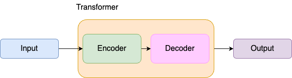
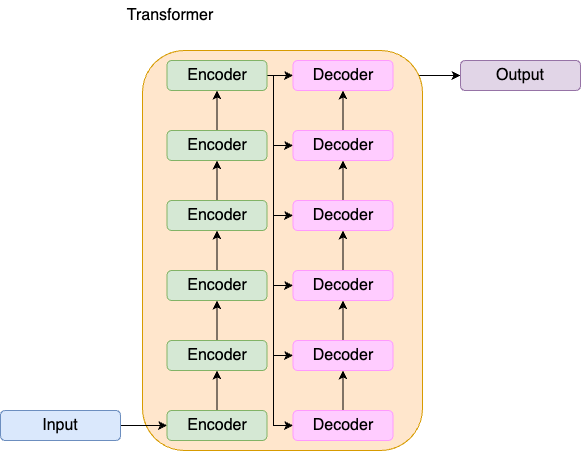
Natural language processing (NLP) is a subfield of artificial intelligence that allows computers to understand, process, and manipulate human language.
Every tool in this course so far needs a vector: \(k\)-means (Lecture 3), \(k\)-nearest neighbours (Lecture 9), regression, SVD and PCA (Lectures 10–13). Text is not a vector. Today is about how text becomes one: text → tokens → vectors.
Learning outcomes. After this lecture you should be able to:
tokenize and normalize text, build a vocabulary and a bag-of-words count matrix;
compute TF, IDF and TF-IDF from the formulas, and say how scikit-learn’s version differs;
compute cosine similarity between documents and use it to retrieve the nearest one;
explain why sparse vectors cannot see synonyms, what an embedding does differently, and how attention makes an embedding depend on its context.
Brief History of NLP and Lecture Outline
NLP Evolution Timeline
1950s-1970s: Rule-Based Era
Turing Test (1950), formal grammars, hand-crafted rules
Systems like ELIZA (1966) - pattern matching “Rogerian therapy” chatbot
# Character and word tokenizationsentence ="Show me the money"word_tokens = sentence.split()print(word_tokens)character_tokens =list(sentence)print(character_tokens)
With tokenization, our goal is to not lose meaning with the tokens. With character based tokenization, especially for English (non-character based languages) we certainly lose meaning.
Huggingface Tokenization
Here is a demo of how to tokenize using the transformers package from Huggingface.
from transformers import AutoTokenizertokenizer = AutoTokenizer.from_pretrained("google-bert/bert-base-cased")tokens = tokenizer.tokenize(sentence)print(tokens)# Try a more advanced sentencesentence2 ="Let's try to see if we can get this transformer to tokenize."tokens2 = tokenizer.tokenize(sentence2)print(tokens2)print("vocabulary size:", tokenizer.vocab_size)
## means “continues the previous token”: token + ##ize = tokenize. BERT’s vocabulary has about 29,000 subwords, and any word can be spelled from them, so the model never meets an unknown word.
Tokens, Token IDs, and Vocabulary
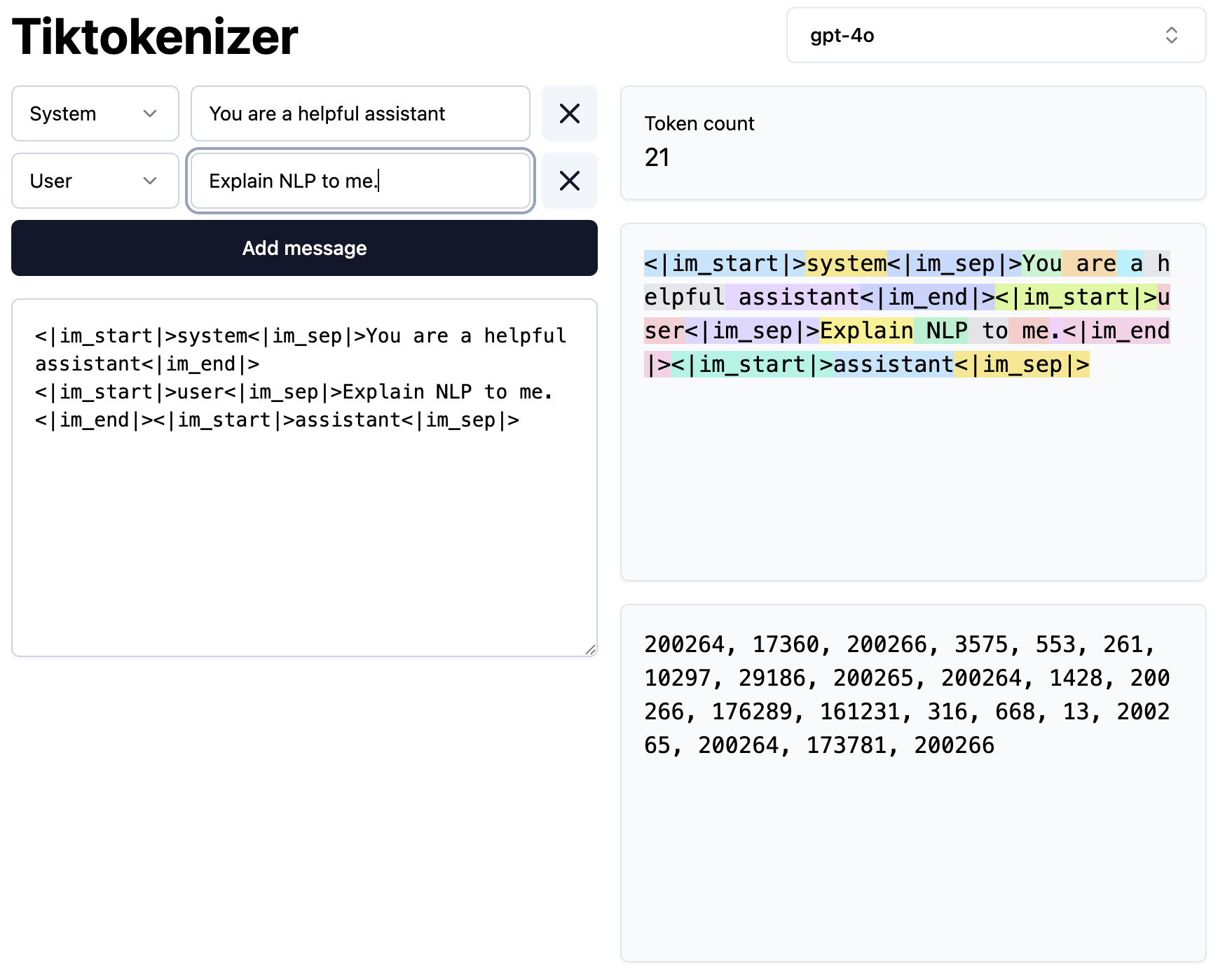
Associated to each token is a unique token ID.
The total number of unique tokens that a model can recognize and process is the vocabulary size.
The vocabulary is the collection of all the unique tokens.
The tokens (and token ids) alone hold no (semantic) information. What is needed is a numerical representation that encodes this information.
There are different ways to achieve this:
One encoding technique that we already considered is one-hot encodings.
Another more powerful encoding method, is the creation of word embeddings.
Before counting words you decide what counts as “the same word”. Each decision changes the vocabulary, and so every column of the matrix you build next.
Lower-case? “The” and “the” become one token.
Strip punctuation? “mat.” and “mat” become one token.
Remove stop words? Drop “the”, “on”, “and”, … from a fixed list.
Stem or lemmatize? A stemmer chops suffixes by rule (Porter: running → run, easily → easili). A lemmatizer looks the word up in a dictionary (ran → run, studies → study).
Stemming vs lemmatization
from nltk.stem import PorterStemmer, WordNetLemmatizerstemmer, lemmatizer = PorterStemmer(), WordNetLemmatizer()print(f"{'word':10}{'stem':10}{'lemma (verb)':12}")for w in ["running", "runs", "ran", "easily", "studies"]:print(f"{w:10}{stemmer.stem(w):10}{lemmatizer.lemmatize(w, pos='v'):12}")
word       stem       lemma (verb)
running    run        run
runs       run        run
ran        ran        run
easily     easili     easily
studies    studi      study
The stemmer is fast and needs no dictionary, but its output need not be a word (easili, studi) and it misses irregular forms (ran).
The lemmatizer returns real words, but needs to know the part of speech: we told it every word is a verb.
Either way, running and runs (and with the lemmatizer ran) collapse into one column.
Sparse Vectors: Counts and TF-IDF
Sparse Representations
You met one-hot encodings for categorical features in Lecture 1.
One-Hot Encoding
Each word is represented as a vector of zeros and a single one.
Simple but inefficient for large vocabularies.
Example
Given the words cat, dog, and emu here are sample one-hot encodings
A document becomes the count of each vocabulary word, ignoring grammar and word order. Three sentences, one row each:
import numpy as npimport pandas as pdfrom sklearn.feature_extraction.text import CountVectorizerdocs = ["The cat sat on the mat.","The dog sat on the log.","The emu sat on the mat."]count_vec = CountVectorizer() # lower-cases, drops punctuationcounts = count_vec.fit_transform(docs).toarray()vocab = count_vec.get_feature_names_out()pd.DataFrame(counts, columns=vocab, index=["S1", "S2", "S3"])
cat
dog
emu
log
mat
on
sat
the
S1
1
0
0
0
1
1
1
2
S2
0
1
0
1
0
1
1
2
S3
0
0
1
0
1
1
1
2
Every decision changes the columns
for options in [{}, {"lowercase": False}, {"stop_words": "english"}]: names = CountVectorizer(**options).fit(docs).get_feature_names_out()print(f"{str(options):28}{len(names)} terms: {list(names)}")
\(\mathrm{tf}\) rewards a term that is frequent in this document.
\(\mathrm{idf}\) rewards a term that is rare across the corpus.
A term in every document has \(\mathrm{idf} = \ln(N/N) = 0\): it is removed automatically, without a stop-word list.
A term in one document gets the largest weight, \(\ln N\).
TF-IDF by hand on the three sentences
With \(N = 3\):
term
df
idf \(= \ln(3/\mathrm{df})\)
the, sat, on
3
\(\ln 1 = 0\)
mat
2
\(\ln 1.5 = 0.405\)
cat, dog, emu, log
1
\(\ln 3 = 1.099\)
Sentence 1: the has tf \(= 2\) but weight \(2 \times 0 = 0\). What is left is cat\(= 1.099\) and mat\(= 0.405\). The words that tell the sentences apart now carry the whole vector.
TF-IDF by hand, in code
The same computation, with counts from the bag-of-words slide:
Smoothing (the \(+1\)s): the gets \(\mathrm{idf}_{\text{sk}} = \ln(4/4) + 1 = 1\), not 0. With tf \(= 2\) it outweighs cat (\(\ln 2 + 1 = 1.69\)). No term is ever weighted exactly 0, and a word that is new at query time cannot cause a division by zero.
\(\ell_2\) normalization: every row has length 1, so long and short documents are comparable and cosine similarity becomes a dot product.
smooth_idf=False removes the \(+1\)s inside the log but keeps the \(+1\) outside, so it is still not the textbook idf.
Practical knobs: stop_words="english", min_df / max_df to prune the vocabulary, sublinear_tf=True for \(1 + \ln \mathrm{tf}\).
On thousands of documents the smoothing barely matters. On three it does.
It measures direction, not length. For counts and TF-IDF (no negative entries) it lies in \([0, 1]\), and 0 means no shared term.
from sklearn.metrics.pairwise import cosine_similarityfor name, X in [("raw counts", counts), ("textbook TF-IDF", tfidf_textbook), ("sklearn TF-IDF", tfidf_sk)]:print(f"cos(S1, S2) on {name:16}: {cosine_similarity(X[[0]], X[[1]])[0, 0]:.2f}")
cos(S1, S2) on raw counts      : 0.75
cos(S1, S2) on textbook TF-IDF : 0.00
cos(S1, S2) on sklearn TF-IDF  : 0.54
Reading the three numbers
Raw counts: \(S_1 \cdot S_2 = 2\cdot 2 + 1 + 1 = 6\) and \(\Vert S_1\Vert^2 = \Vert S_2\Vert^2 = 8\), so \(6/8 = 0.75\). “Similar” only because both contain the, sat, on.
Textbook TF-IDF: the only shared terms have idf 0, so the cat sentence and the dog sentence are orthogonal.
sklearn’s smoothing keeps a little of the, sat, on: 0.54.
Retrieval: a search engine in one line
The most relevant document for a query \(q\) is \(\arg\max_j \cos(q, d_j)\).
query = ["the dog on the mat"]for name, vec in [("raw counts", count_vec), ("sklearn TF-IDF", tfidf_vec)]: sims = cosine_similarity(vec.transform(query), vec.transform(docs))[0]print(f"{name:15} similarities {sims.round(3)} -> best: S{sims.argmax() +1}")
On raw counts all three sentences tie: the and on decide everything. TF-IDF breaks the tie on the informative word, dog. (np.argmax returns the first of a tie, so “S1” on the first line is an accident.)
Word Embeddings
Word Embeddings
Word embeddings represent words as dense vectors in high-dimensional spaces.
The individual values of the vector may be difficult to interpret, but the overall pattern is that words with similar meanings are close to each other, in the sense that their vectors have small angles with each other.
Question: Is that true with one-hot encodings?
Answer: No, with one-hot encodings, the similarity of two words is 0 if they are different, and 1 if they are the same.
The same holds for bag of words and TF-IDF: every word is its own axis, so “doctor” and “physician” are orthogonal and two documents look similar only if they share literal words.
The similarity of two word embeddings is again the cosine of the angle between them.
Static vs Contextual Embeddings
Word embeddings can be static or contextual.
Static: A static embedding is when each word has a single embedding, e.g., Word2Vec.
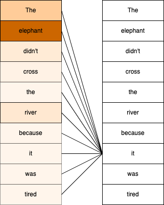
Contextual: A contextual embedding (used by more complex language model embedding algorithms) allows the embedding for a word to change depending on its context in a sentence.
Word2Vec: Static Embeddings
Word2Vec(Mikolov et al. 2013) is a technique to learn static word embeddings from large text corpora.
Key characteristics:
Each word has a single fixed vector representation
Trained to predict a word from its context (CBOW) or the context from a word (Skip-gram)
Captures semantic relationships: king - man + woman ≈ queen
Popular pre-trained model: Google News (300d). Related: GloVe, which is count-based (it factorizes global word co-occurrence counts) rather than predictive
Advantages:
Fast to train and use
Efficient for large vocabularies
Good for similarity tasks, clustering
Pre-trained embeddings available
Disadvantages:
Limited context and no word order information.
For phrases and sentences, the embedding is the average of the word embeddings.
Contextual vs Static Embeddings
Feature
Static (Word2Vec, GloVe)
Contextual (BERT, GPT)
Representation
One vector per word
Different vectors per context
Example
“bank” always same vector
“bank” differs in “river bank” vs “bank account”
Model Type
Shallow model
Deep transformer model
Training
Fast, lightweight
Slow, resource-intensive
Best For
Similarity, clustering, simple tasks
Complex understanding, ambiguity resolution
Dimensionality
100-300 dimensions
768-1024+ dimensions
When to use Word2Vec:
Limited computational resources
Task doesn’t require deep context understanding
Working with domain-specific corpora (train custom embeddings)
When to use Contextual Embeddings:
Need to handle polysemy (words with multiple meanings)
A language model is a statistical tool that predicts the probability of a sequence of words. It helps in understanding and generating human language by learning patterns and structures from large text corpora.
N-gram Models:
Predict the next word based on the previous \(n-1\) words.
Simple and effective for many tasks but limited by fixed context size.
Neural Language Models:
Use neural networks to capture more complex patterns.
Common uses: Text completion, creative writing, chatbots, code generation
Transformer Applications
Transformers enable powerful NLP applications:
Machine Translation: Translate between languages
Text Summarization: Generate concise summaries
Question Answering: Answer questions from context
Named Entity Recognition: Identify entities in text
Sentiment Analysis: Determine sentiment/emotion
Text Generation: Create human-like text
NLP Packages Overview
NLTK: Natural Language Toolkit
NLTK is one of the most comprehensive Python libraries for NLP, created for teaching and research.
Key Features:
Extensive text processing tools (tokenization, stemming, tagging, parsing)
Access to 50+ corpora and lexical resources (WordNet, TreeBank)
Sentiment analysis, text classification, and chunking
Best For:
Learning classical NLP concepts and fundamentals
Academic research and prototyping
Working with linguistic data structures
Access to curated corpora
Limitations:
Slower than modern libraries
Less suited for production
Requires more manual pipeline construction
spaCy: Production-Ready NLP
spaCy is a modern, industrial-strength NLP library designed for production use.
Key Features:
Fast and efficient (Cython-optimized)
Tokenization for 75+ languages, trained pipelines for about 25
Built-in NER, POS tagging, dependency parsing
Word vectors and document similarity
Beautiful visualization tools (displaCy)
Easy integration with deep learning (PyTorch, TensorFlow)
Best For:
Production NLP pipelines
Real-time text processing
Information extraction at scale
Named Entity Recognition
Document analysis and classification
LangChain: Overview
LangChain(Chase 2022) is a framework for building applications on top of large language models.
One interface to many model providers, so the model can be swapped without rewriting the application
Chains prompts, model calls, document retrieval and tool calls into one pipeline
Typical uses: chatbots over your own documents (retrieval-augmented generation), information extraction, summarization
Retrieval-augmented generation retrieves the documents nearest the question, as on the retrieval slide above but usually with dense embeddings, and hands them to the language model.
Where the code lives
Runnable examples of every package on these slides (NLTK preprocessing and sentiment, the spaCy pipeline and NER, BERTopic with its visualizations, and a LangChain pointer) are in Appendix A5: NLP Packages, which also has a Colab notebook.
The rest of this lecture looks at two applications: named entity recognition and topic modeling.
Named Entity Recognition (NER)
What is Named Entity Recognition?
Named Entity Recognition (NER) is the task of identifying and classifying named entities in text into predefined categories.
Applications: Information extraction, content classification, question answering, knowledge graphs
NER with spaCy
spaCy’s small English pipeline (en_core_web_sm) tags one sentence pair:
Apple Inc.
ORG
was founded by
Steve Jobs
PERSON
in
Cupertino
GPE
,
California
GPE
, in
1976
DATE
. It reported revenue of
$391 billion
MONEY
in
fiscal 2024
DATE
.
One call runs the whole pipeline: tokenizer → tagger → parser → lemmatizer → NER.
The NER component is a trained model, not a list of names: “fiscal 2024” is a DATE because of how it is used.
The code, entity attributes and the pipeline components are in Appendix A5.
Topic Modeling
What is Topic Modeling?
Topic modeling is an unsupervised learning technique that discovers abstract “topics” in a collection of documents.
Key concepts:
Topic: A distribution over words (e.g., “sports” → {game, team, player, score, …})
Document: A mixture of topics
Goal: Automatically discover topics and their distributions
Applications:
Content recommendation and discovery
Document organization and clustering
Trend analysis over time
Search and information retrieval
Content summarization
Classical approaches (LDA, NMF) use bag-of-words representations and require specifying the number of topics.
Modern approaches (BERTopic) cluster transformer embeddings; the clustering step decides how many topics there are, given a minimum topic size.
BERTopic: Overview
BERTopic(Grootendorst 2022) is a modern topic modeling technique using transformer embeddings.
Key advantages:
Uses semantic embeddings from a transformer (captures context and meaning)
HDBSCAN chooses the number of topics, given min_topic_size
Works on short documents (tweets, reviews, titles)
Built-in interactive visualizations
What it still needs from you:
A stop-word list for the topic words (it is TF-IDF underneath)
A choice of min_topic_size, which sets how fine the topics are
Reading the topics: some will be junk
A GPU for large corpora
BERTopic: How It Works
BERTopic uses a modular pipeline with four main steps:
1. Document Embeddings
Use a pre-trained sentence-transformer model
Each document → a dense vector (384 dimensions for all-MiniLM-L6-v2, 768+ for larger models)
Concatenate each cluster’s documents into one “document” and run TF-IDF over the clusters
Extracts most representative words per topic
Creates interpretable topic labels
BERTopic on three newsgroups
The same three newsgroups we clustered in Lecture 4:
BERTopic setup and fit (full walkthrough in Appendix A5)
from bertopic import BERTopicfrom sentence_transformers import SentenceTransformerfrom sklearn.datasets import fetch_20newsgroupsfrom umap import UMAPcategories = ['comp.os.ms-windows.misc', 'sci.space', 'rec.sport.baseball']posts = fetch_20newsgroups(subset='all', categories=categories, remove=('headers', 'footers', 'quotes'))['data']posts = [p for p in posts iflen(p.split()) >=5] # drop empty postsembedder = SentenceTransformer("all-MiniLM-L6-v2")embeddings = embedder.encode(posts, show_progress_bar=False) # step 1, computed oncedef fit_bertopic(min_topic_size): model = BERTopic( embedding_model=embedder, umap_model=UMAP(n_neighbors=15, n_components=5, min_dist=0.0, metric="cosine", random_state=42), vectorizer_model=CountVectorizer(stop_words="english", token_pattern=r"(?u)\b[a-zA-Z]{3,15}\b"), min_topic_size=min_topic_size) topics, _ = model.fit_transform(posts, embeddings)return model, topicsfor size in (20, 10): model, topics = fit_bertopic(size)print(f"min_topic_size={size}: {len(set(topics) - {-1})} topics, "f"{topics.count(-1)} outliers out of {len(posts)} posts")
min_topic_size=20: 3 topics, 0 outliers out of 2823 posts
min_topic_size=10: 21 topics, 285 outliers out of 2823 posts
With min_topic_size=20 HDBSCAN finds exactly the three newsgroups, without ever seeing a label. Halve it and the same embeddings give 21 topics. The number of topics is a consequence of the minimum size you ask for, not a property of the data alone.
BERTopic: the topics
With min_topic_size=10 we get many small topics; reduce_topics merges the most similar ones until 10 remain (the outlier row −1 counts as one).
topic_model = modeltopic_model.reduce_topics(posts, nr_topics=10)info = topic_model.get_topic_info()info["Top words"] = [", ".join(w for w, _ in topic_model.get_topic(t)[:5]) for t in info.Topic]print(info[["Topic", "Count", "Top words"]].to_string(index=False))
Space and baseball stay whole. Windows splits into drivers, printers, fonts, sound and disks. Topic 7 is junk (posts of encoded binary files), and the 285 outliers are mostly Windows posts. Always read your topics.
Each circle is a topic, sized by its number of posts, placed by the similarity of the topics’ c-TF-IDF vectors.
Summary
What you should now be able to do
Text → tokens → vectors. Tokenize (characters, words, subwords); every preprocessing decision (case, punctuation, stop words, stem or lemma) changes the vocabulary.
TF-IDF\(= \mathrm{tf} \times \ln(N/\mathrm{df})\): frequent here, rare overall. A term in every document gets 0. scikit-learn smooths the idf and \(\ell_2\)-normalizes the rows, which is why the = 0.6165 survives in its table.
Cosine similarity compares direction. On the three sentences: 0.75 on counts, 0 on textbook TF-IDF, 0.54 on sklearn’s. Retrieval is \(\arg\max_j \cos(q, d_j)\).
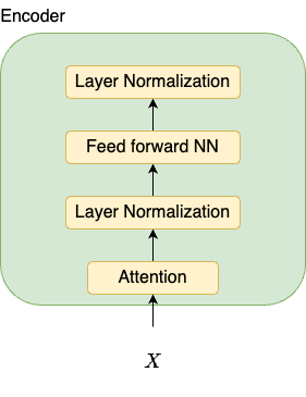
Sparse vs dense. Sparse vectors see shared words, not synonyms. Embeddings learn dense vectors where similar meaning means a small angle; attention makes them depend on context (QKV, softmax-weighted sum). BERT encodes, GPT generates.
Tools. NLTK and spaCy for preprocessing and NER; BERTopic = embed → UMAP → HDBSCAN → c-TF-IDF; runnable examples in Appendix A5.
References
Brown, Tom B, Benjamin Mann, Nick Ryder, et al. 2020. “Language Models Are Few-Shot Learners.”arXiv Preprint arXiv:2005.14165, ahead of print. https://doi.org/10.48550/arXiv.2005.14165.
Devlin, Jacob, Ming-Wei Chang, Kenton Lee, and Kristina Toutanova. 2019. “BERT: Pre-Training of Deep Bidirectional Transformers for Language Understanding.”arXiv Preprint arXiv:1810.04805, ahead of print. https://doi.org/10.48550/arXiv.1810.04805.
Grootendorst, Maarten. 2022. “BERTopic: Neural Topic Modeling with a Class-Based TF-IDF Procedure.”arXiv Preprint arXiv:2203.05794. https://arxiv.org/abs/2203.05794.
Mikolov, Tomas, Kai Chen, Greg Corrado, and Jeffrey Dean. 2013. “Efficient Estimation of Word Representations in Vector Space.”Proceedings of Workshop at ICLR. https://arxiv.org/abs/1301.3781.
Vaswani, Ashish, Noam Shazeer, Niki Parmar, et al. 2017. “Attention Is All You Need.”Proceedings of the 31st Conference on Neural Information Processing Systems (NIPS 2017) (Long Beach, CA, USA), 11. https://arxiv.org/abs/1706.03762.