Recap: Neural Networks II — Making Training Work
DS701 Session 20 — Wed Nov 11, 2026


Today’s plan
- 5 min — knowledge-check review
- 20 min — highlights and Q&A (answer or pass — answering always earns credit)
- 30 min — case study: reading handwritten form fields on a budget
- wrap-up and cold-call check-ins
Knowledge-Check Review
KC 1: The knobs
The lecture maps the ideas from Neural Networks I onto MLPClassifier arguments. Name the scikit-learn argument that sets each of the following, and say in one phrase what a larger value does: (a) the number of layers and neurons per layer, (b) the learning rate, (c) the mini-batch size, (d) the maximum number of epochs, (e) the strength of L2 regularization. Which solver does the lecture recommend as the default?
KC 2: What the loss curve does — and does not — tell you
After training the MNIST model, the lecture plots mlp.loss_curve_: a fast drop, then a smooth flattening. What exactly is being plotted (which data, which quantity), and why does a smoothly decreasing curve of that kind not by itself guarantee good performance on the test set? Which two MLPRegressor arguments in the California-housing example address that concern, and how?
KC 3: “Because neural networks”
A colleague has 8,000 rows of tabular customer data with 25 numeric features and wants to build the classifier in PyTorch “because neural networks.” Using the lecture’s scikit-learn-vs-PyTorch/TensorFlow criteria, what would you recommend and why? Name two things about the problem that would change your recommendation, and one preprocessing step you would insist on either way.
Highlights
Every idea from last time is now an argument
| Concept (NN I) | scikit-learn |
|---|---|
| layers and neurons | hidden_layer_sizes |
| activation \(f\) | activation |
| learning rate \(\eta\) | learning_rate_init |
| mini-batch size | batch_size |
| optimizer | solver — adam / sgd / lbfgs |
| epochs / stopping | max_iter, early_stopping, n_iter_no_change |
| regularization | alpha (L2) |
- Start simple: one hidden layer, sizes between the input and output dimension; add depth only when the data can pay for it.
- Input and output sizes come from the data — you never set them.
max_iteris a ceiling, not a target: adam stops when the training loss stalls forn_iter_no_changeepochs.adamforgives a mediocre learning rate;sgddoes not.
Standardize inputs. Always.
Gradient descent takes one step size for every direction. If one feature spans 0–4000 and another 0–0.2, that feature dominates every weighted sum and every gradient, the loss surface is a long narrow valley, and no single learning rate suits both.
- MNIST: pixels / 255 → \([0, 1]\).
- Housing:
StandardScaler→ zero mean, unit variance per feature. The lecture’s raw-feature fit started at a loss of ~30,000 and reached test \(R^2\) 0.45; standardized, 0.76. - Fit the scaler on the training split only;
transformthe test split with it. Fitting on everything leaks test statistics into training. - Best done inside a
Pipeline([('scaler', StandardScaler()), ('mlp', MLPClassifier(...))])so cross-validation and grid search re-fit it correctly per fold.
When it barely matters: features already on one common scale (pixels).
When it rescues you: real measurements with wildly different units — the difference between a model that works and one that flails.
Today’s case study trains on sklearn’s 8×8 digits — the vendor’s form fields.
Read the loss curve before you read the accuracy
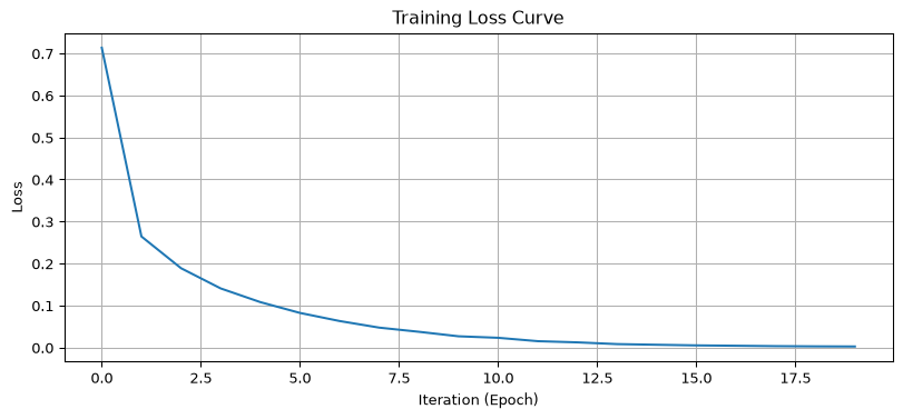
One point = training loss after one epoch. Healthy: fast initial drop, smooth flattening. It was still falling at max_iter=20 — that is all the ConvergenceWarning meant.
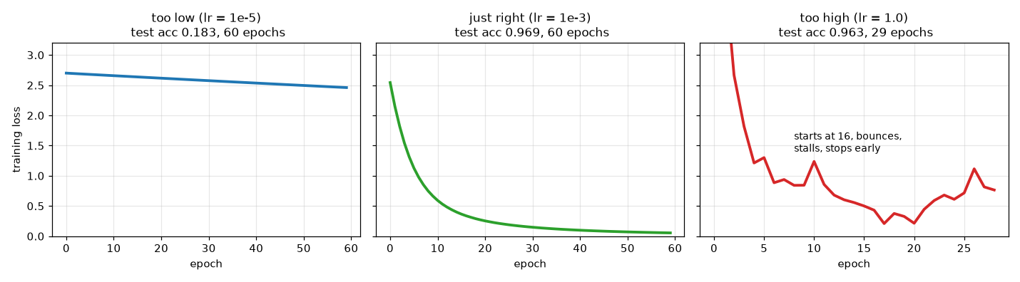
Too low: barely moves. Too high: starts absurdly high, bounces, stalls, and stops “because it stopped improving”. The right-hand model happened to score well — would you ship it?
Overfitting: what the loss curve cannot show you
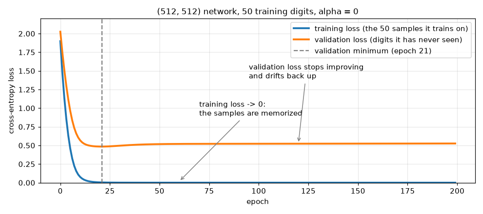
- A
(512, 512)network has ~300K weights; 50 training digits cannot pin them down. Training loss → 0 — the samples are memorized. - Loss on data the model has never seen bottoms out around epoch 20 and drifts back up. Everything after the dashed line is fitting noise.
- You only see this if you hold data out and measure it —
loss_curve_alone would have said “learning nicely”.
Diagnose, then repair
Diagnose with data the optimizer never saw — a validation split, or cross-validation (cross_val_score, GridSearchCV). That is a measurement; it changes nothing about the model.
| repair | scikit-learn | what it changes |
|---|---|---|
| L2 regularization | alpha=0.01 (default 1e-4) |
the objective: penalizes large weights |
| early stopping | early_stopping=True, validation_fraction=0.1, n_iter_no_change=10 |
the training loop: stop on validation evidence, not training loss |
| smaller network | e.g. (64,) instead of (512, 512) |
the capacity: fewer weights to memorize with |
| more data | more training rows | the information: more constraints per weight |
Regularizers trade variance for bias; only more data creates information.
Early stopping is not free either — it takes validation_fraction of your training data away. Ask what that costs when the training set is tiny.
The case study’s report-out asks which of these levers you would pull first for the vendor’s reader, and why.
Tuning honestly
GridSearchCV(mlp, param_grid, cv=3)— every configuration × every fold is a full training run: \(3 \text{ architectures} \times 2\ \alpha \times 3 \text{ folds} = 18\) fits before the refit. Budget accordingly (the lecture used 1,500 samples for the demo).- Tune on the folds, never on the test set; the test set is spent once, at the end.
- Read
cv_results_— the spread (std_test_score) tells you whether the “best” setting is really better or just lucky. In the lecture’s grid, five of six configurations were within one std (0.0075) of the best. - Solvers on the same budget (2,000 digits, 50 epochs):
adam0.90,lbfgs0.88,sgd0.83 — the one that lost had simply not converged yet.
When the toy tool is enough
scikit-learn MLPClassifier / MLPRegressor
- small–medium tabular data (< ~100K rows)
- standard feed-forward architectures
- CPU training is fine
- lives inside
Pipeline,cross_val_score,GridSearchCV - fastest way to a tuned baseline — and to a fair comparison with logistic regression, trees, kNN
PyTorch / TensorFlow
- large data, GPUs, data that does not fit in memory
- CNNs, RNNs, transformers, custom losses
- production and research
Depth on those architectures lives in the optional modules M4 (CNNs) and M3 (RNNs), and in a dedicated course — DS542, Deep Learning for Data Science. In DS701 the point is to train a network correctly and know when you have.
In-Class Activity
Activity — Case Study 17: Reading Handwritten Form Fields on a Fixed Training Budget
Goal: a vendor that digitizes handwritten clinic intake forms wants a digit reader trained on a laptop within a fixed epoch budget, and wants to know what to do on the day it starts memorizing their scans. Prototyping on scikit-learn’s 8×8 digits (their own scans are not released yet), you run the lecture’s recipe — standardize, fit, read the loss curve, score on held-out data (Part 1) — then give two solvers × two learning rates the same 50-epoch budget and pick the combination that earns it (Part 2). The report-out is your memo to the vendor: the recommendation, and the caveat — how they would diagnose memorization from the train-vs-validation loss picture, and which of the four repairs (alpha, early stopping, a smaller network, more data) to pull first.
- Work in groups of 2–3. Open your section’s notebook.
- Parts marked (autograded) are submitted to Gradescope; the rest is participation.
- Staff will circulate — be ready to explain any part of your work.
- Dependencies:
numpy,matplotlib,scikit-learn. Every fit takes well under a second.


The activity notebook goes live on the day of the lecture. Colab is optional — you can also open it on GitHub and run it locally.
Going deeper
Full lecture notes: Neural Networks II: Making Training Work
- Today: The Knobs — the concept-to-argument table
- Prepare the Data and Data Preprocessing — scaling, and the
Pipelinepattern - Training Loss Curve — the MNIST curve and its
ConvergenceWarning; Common Issues — convergence remedies matched to the curve - Prepare Data and Define Model and Training and Validation Curves — early stopping in the housing regressor
- Why Scaling Matters — standardized vs raw housing features
- Reading the Learning Rate from the Loss Curve and Overfitting: What the Training Curve Cannot Show
- Overfitting: Diagnose, Then Repair — validation and CV measure;
alpha, early stopping, a smaller network and more data repair - Grid Search for Optimal Architecture and Solver Selection
- Scikit-Learn vs PyTorch/TensorFlow and What scikit-learn’s MLP Cannot Do
- Last session’s theory: Neural Networks I: How Learning Works; deeper dives: Gradient Descent, Backpropagation, SGD, batches and CNNs, RNNs, Neural Networks with scikit-learn: advanced features