Recap: Distances, Norms and Similarity
DS701 Session 3 — Mon Sep 14, 2026


Today’s plan
- 5 min — knowledge-check review
- 20 min — highlights and Q&A (answer or pass — answering always earns credit)
- 60 min — in-class activity (small groups)
- wrap-up and cold-call check-ins
Knowledge-Check Review
KC 1: What makes a metric?
State the four properties a function \(d(x, y)\) must satisfy to be called a metric. Then say, in one line, how a norm \(p(\cdot)\) gives you a metric for free.
Show answer
Answer:
- \(d(x, x) = 0\)
- \(d(x, y) > 0\) for all \(x \neq y\) (positivity)
- \(d(x, y) = d(y, x)\) (symmetry)
- \(d(x, y) \le d(x, z) + d(z, y)\) (triangle inequality)
Every norm induces a metric: \(d(\mathbf{x}, \mathbf{y}) = p(\mathbf{x} - \mathbf{y})\). \(\ell_2 \to\) Euclidean, \(\ell_1 \to\) Manhattan, \(\ell_\infty \to\) Chebyshev. The converse fails: the discrete metric (\(0\) if equal, else \(1\)) comes from no norm.
KC 2: Inner products, norms, angles
Let \(\mathbf{u} = [1, 2, 0]\) and \(\mathbf{v} = [3, -1, 4]\).
Compute
- the inner product \(\mathbf{u}\cdot\mathbf{v}\),
- \(\Vert\mathbf{u}\Vert_2\) and \(\Vert\mathbf{v}\Vert_2\),
- the cosine of the angle between them, and
- the \(\ell_1\) and \(\ell_\infty\) distances \(\Vert\mathbf{u}-\mathbf{v}\Vert_1\), \(\Vert\mathbf{u}-\mathbf{v}\Vert_\infty\).
Then explain in one sentence why the cosine can be near one while the vectors are far apart in every \(\ell_p\) distance.*
Show answer
Answer:
- \(\mathbf{u}\cdot\mathbf{v} = 1\cdot 3 + 2\cdot(-1) + 0\cdot 4 = 1\)
- \(\Vert\mathbf{u}\Vert_2 = \sqrt{5}\), \(\quad \Vert\mathbf{v}\Vert_2 = \sqrt{26}\)
- \(\cos\theta = 1/\sqrt{130} \approx 0.09\) — nearly orthogonal
- \(\mathbf{u} - \mathbf{v} = [-2, 3, -4]\): \(\ \Vert\cdot\Vert_1 = 9\), \(\ \Vert\cdot\Vert_\infty = 4\) (and \(\Vert\cdot\Vert_2 = \sqrt{29} \approx 5.4\) in between)
Cosine measures direction only — rescale either vector and it does not move. An \(\ell_p\) distance measures the length of the difference vector, so magnitude matters. Nearly parallel and far apart is perfectly consistent.
KC 3: Hamming vs. Jaccard
Two situations from the lecture.
- Case 1: two long documents, almost identical, that differ in 10 words.
- Case 2: two 5-word documents with no words in common. Represent each document as a bit vector over the vocabulary.
What is the Hamming distance in each case, why does that ranking feel wrong, and which measure from the lecture fixes it (give its formula)?*
Show answer
Answer: Hamming \(= \ell_1\) on bit vectors \(=\) size of the set difference: Case 1 \(= 10\), Case 2 \(= 5\). So Hamming calls the near-identical long documents more different than two documents that share nothing — it counts raw disagreements without normalizing by how much there was to agree on.
Jaccard fixes it: \[ J_{sim}(x, y) = \frac{|x \cap y|}{|x \cup y|} \qquad \approx 1 \text{ in Case 1},\quad 0 \text{ in Case 2}. \] \(1 - J_{sim}\) is a genuine metric. Lesson: the right distance depends on what the data represents.
Highlights
Linear-algebra essentials
Everything today lives in \(\mathbb{R}^d\): a data object is a vector \(\mathbf{x} = [x_1, \dots, x_d]\), a dataset is an \(m \times d\) matrix (rows = objects, columns = features).
Inner product — elementwise multiply, then sum: \[\mathbf{u}\cdot\mathbf{v} = \mathbf{u}^T\mathbf{v} = \sum_i u_i v_i\]
Norm — a length. The \(\ell_2\) norm is the one you know: \[\Vert\mathbf{v}\Vert_2 = \sqrt{\mathbf{v}\cdot\mathbf{v}} = \sqrt{\textstyle\sum_i v_i^2}\]
Distance — the norm of the difference: \[d(\mathbf{u},\mathbf{v}) = \Vert\mathbf{u} - \mathbf{v}\Vert\]
Cosine of Angle — inner product with the lengths divided out: \[\cos\theta = \frac{\mathbf{u}\cdot\mathbf{v}}{\Vert\mathbf{u}\Vert_2\,\Vert\mathbf{v}\Vert_2}\]
- \(\mathbf{u}\cdot\mathbf{v} = 0 \iff\) orthogonal
- unit vector: \(\mathbf{v}/\Vert\mathbf{v}\Vert_2\) has length 1
- one-hot categories are unit vectors, mutually orthogonal — that is why we one-hot rather than number the levels 1, 2, 3
What makes a metric
A metric \(d(x,y)\) satisfies
- \(d(x, x) = 0\)
- \(d(x, y) > 0 \quad \forall x \neq y\) (positivity)
- \(d(x, y) = d(y, x)\) (symmetry)
- \(d(x, y) \le d(x, z) + d(z, y)\) (triangle inequality)
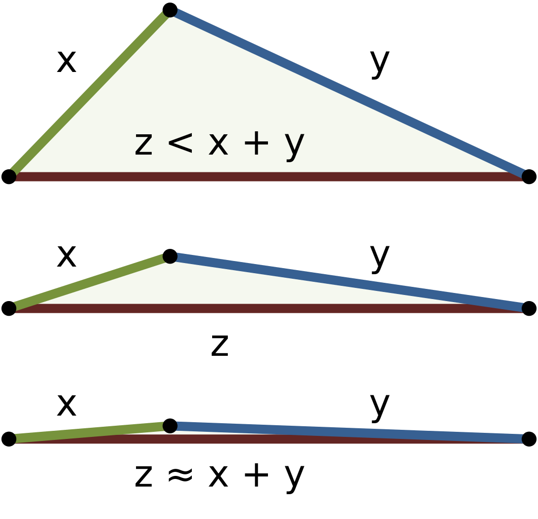
A metric measures dissimilarity: bigger \(=\) more different. On vectors we call it a distance. Symmetry and the triangle inequality are what let us reason about “neighborhoods” — nearest-neighbor search, clustering, and everything downstream leans on them.
Not everything we call a “distance” is one: \(1 - \cos(\mathbf{x},\mathbf{y})\) is not a metric. We will still use it, but we will say dissimilarity.
Norm \(\to\) metric: the \(\ell_p\) family
A norm \(p(\mathbf{v})\): \(p(a\mathbf{v}) = |a|\,p(\mathbf{v})\), \(\ p(\mathbf{u}+\mathbf{v}) \le p(\mathbf{u}) + p(\mathbf{v})\), \(\ p(\mathbf{v}) = 0 \iff \mathbf{v} = 0\).
Every norm gives a metric: \(d(\mathbf{x},\mathbf{y}) = p(\mathbf{x} - \mathbf{y})\).
\[ \Vert \mathbf{x} - \mathbf{y} \Vert_p = \Big(\sum_{i=1}^d |x_i - y_i|^p\Big)^{1/p}, \qquad p \ge 1 \]
| \(p\) | norm | distance |
|---|---|---|
| \(1\) | \(\sum_i \lvert x_i - y_i \rvert\) | Manhattan (Hamming on bits) |
| \(2\) | \(\sqrt{\sum_i (x_i - y_i)^2}\) | Euclidean |
| \(\infty\) | \(\max_i \lvert x_i - y_i \rvert\) | Chebyshev / maximum |
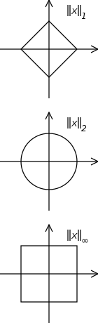
The unit “circles”: diamond \(\subset\) circle \(\subset\) square, because \(\Vert\cdot\Vert_1 \ge \Vert\cdot\Vert_2 \ge \Vert\cdot\Vert_\infty\).
Which \(\ell_p\) is right?
The choice of \(p\) decides what gets emphasized.
\(\ell_1\) — Manhattan
- many small differences count
- robust to a single large one
- natural for sparse data, counts, bit vectors
\(\ell_2\) — Euclidean
- the default in geometric space
- smooth, differentiable, rotation-invariant
- squares → outliers hurt more than in \(\ell_1\)
\(\ell_\infty\) — Chebyshev
- only the largest difference counts
- extremely outlier-sensitive
- right when you need a uniform bound
Same two points, three different answers: \(A=(3,4)\), \(B=(1,1)\) gives \(5\), \(\sqrt{13}\), \(3\). The ranking of neighbors can change with \(p\) — that is the point, not a nuisance.
Cosine vs. Euclidean
Cosine similarity — the angle, lengths divided out: \[ \cos(\mathbf{x},\mathbf{y}) = \frac{\mathbf{x}^T\mathbf{y}}{\Vert\mathbf{x}\Vert\,\Vert\mathbf{y}\Vert} \]
- \(1\) same direction, \(0\) orthogonal
- scale-invariant: \(\cos(\mathbf{x}, 2\mathbf{y}) = \cos(\mathbf{x},\mathbf{y})\)
- dissimilarity: \(1 - \cos(\mathbf{x},\mathbf{y})\) — not a metric
Euclidean distance — the length of the gap: \[ \Vert\mathbf{x} - \mathbf{y}\Vert_2 \]
- \(0\) only when identical
- scale-sensitive: doubling \(\mathbf{y}\) moves it
- a metric
Word-count vectors: document B \(=\) document A pasted twice. Cosine says identical (\(1\)); Euclidean says far (\(\Vert\mathbf{A}\Vert\)). For text we usually want the proportions, not the length → cosine.
Rule of thumb: ask “do I care about magnitude?” If not, cosine (or normalize to unit length first, after which Euclidean and cosine rank neighbors identically).
Why scaling matters
The units of each feature are part of the model. Wine dataset, 13 chemical measurements:
| feature | typical range | std. dev. |
|---|---|---|
hue |
0.5 – 1.7 | 0.23 |
alcohol |
11 – 15 | 0.81 |
magnesium |
70 – 160 | 14 |
proline |
280 – 1680 | 314 |
Raw Euclidean distance between two wines \(\approx |\Delta\,\texttt{proline}|\): proline alone carries \(99.7\%\) of the total variance. Twelve features are invisible.
Standardize — per feature, subtract the mean and divide by the standard deviation — and the nearest neighbors change. In the activity you will measure exactly how much (spoiler: 1-NN accuracy on the wine type goes from ~0.65 to ~1.0).
Two separate decisions, both yours: which metric, and which units. Cosine does not rescue you from bad units — the direction is still dominated by the big coordinate.
Sets and bit vectors: Hamming vs. Jaccard
Bit vector as a code (every position matters): Hamming \(= \ell_1 =\) number of bit flips.
Bit vector as a set (which items are present): Hamming counts the set difference, and that misleads — 10 differing words out of thousands beats 5 disjoint words.
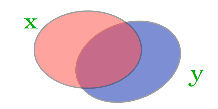
Jaccard normalizes by how much there was to agree on: \[ J_{sim} = \frac{|x \cap y|}{|x \cup y|}, \qquad J_{dist} = 1 - J_{sim} \ \text{ (a metric)} \]
| data | first choice |
|---|---|
| real measurements, comparable units | Euclidean (\(\ell_1\) if outliers) — standardize first |
| word counts, varying lengths | cosine |
| item sets / baskets | Jaccard |
| aligned binary codes | Hamming |
In-Class Activity
Activity: Distance matrices, by hand and with scikit-learn
Goal: build Euclidean, Manhattan, cosine and Jaccard distance matrices on real data with numpy, verify them against sklearn / scipy, watch nearest neighbors change with the metric and with feature scaling.
- Work in groups of 2–3.
- Parts marked (autograded) are submitted to Gradescope; the rest is participation.
- Staff will circulate — be ready to explain any part of your work.
- Dependencies:
numpy,pandas,matplotlib,scipy,scikit-learnonly.


The activity notebook goes live on the day of the lecture. Colab is optional — you can also open it on GitHub and run it locally.
Going deeper
Full lecture notes: Distances and Time Series
- Feature space representation — one-hot encoding and why not 1, 2, 3
- Metrics — the four axioms and the distance matrix
- Norms and the \(\ell_p\) family — Minkowski distance, \(\ell_1\), \(\ell_2\), \(\ell_\infty\), and the not-a-norm \(\ell_0\)
- Similarity and dissimilarity — cosine and how to turn a similarity into a dissimilarity
- Bit vectors and sets — Hamming and Jaccard
- Linear-algebra background: dot product and \(\ell_2\) norm, definitions: unit vector, distance, angle
- The
sklearnfit/transformAPI: Scikit-Learn appendix - Time series and dynamic time warping in full: optional module M2 Time Series (and the DTW section of this lecture)