
Code
import numpy as np
import matplotlib.pyplot as plt
import pandas as pd
import seaborn as sns
from IPython.display import Image, HTML
from slideUtilities import OKABE_ITO
import warnings
warnings.filterwarnings('ignore')

%matplotlib inline


import numpy as np
import matplotlib.pyplot as plt
import pandas as pd
import seaborn as sns
from IPython.display import Image, HTML
from slideUtilities import OKABE_ITO
import warnings
warnings.filterwarnings('ignore')
%matplotlib inlineThis is the first of two lectures on neural networks. Today is about how learning works: we build the model up from regression, define what “training” means, and then look carefully at the machinery that makes it possible.
We’ll cover:
Next lecture, Neural Networks II, is about making training work in practice with scikit-learn.
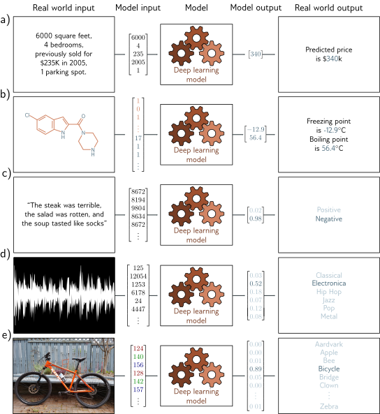
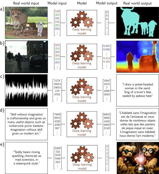
Neural networks are the model family behind essentially all of modern computer vision, speech, and language systems, and are competitive on tabular data too.
Recall linear regression predicts a continuous output:
\[ \hat{y} = \beta_0 + \beta_1 x_1 + \beta_2 x_2 + \cdots + \beta_p x_p = \mathbf{x}^T\boldsymbol{\beta} \]
Or in matrix form for multiple samples:
\[ \hat{\mathbf{y}} = \mathbf{X}\boldsymbol{\beta} \]
Question: What’s the main limitation of linear regression?
Answer: It can only model linear relationships between inputs and outputs!
Adds Non-linearity
For binary classification, logistic regression applies a sigmoid function:
\[ P(y=1|\mathbf{x}) = \sigma(\mathbf{x}^T\boldsymbol{\beta}) = \frac{1}{1 + e^{-\mathbf{x}^T\boldsymbol{\beta}}} \]
The sigmoid function introduces non-linearity:
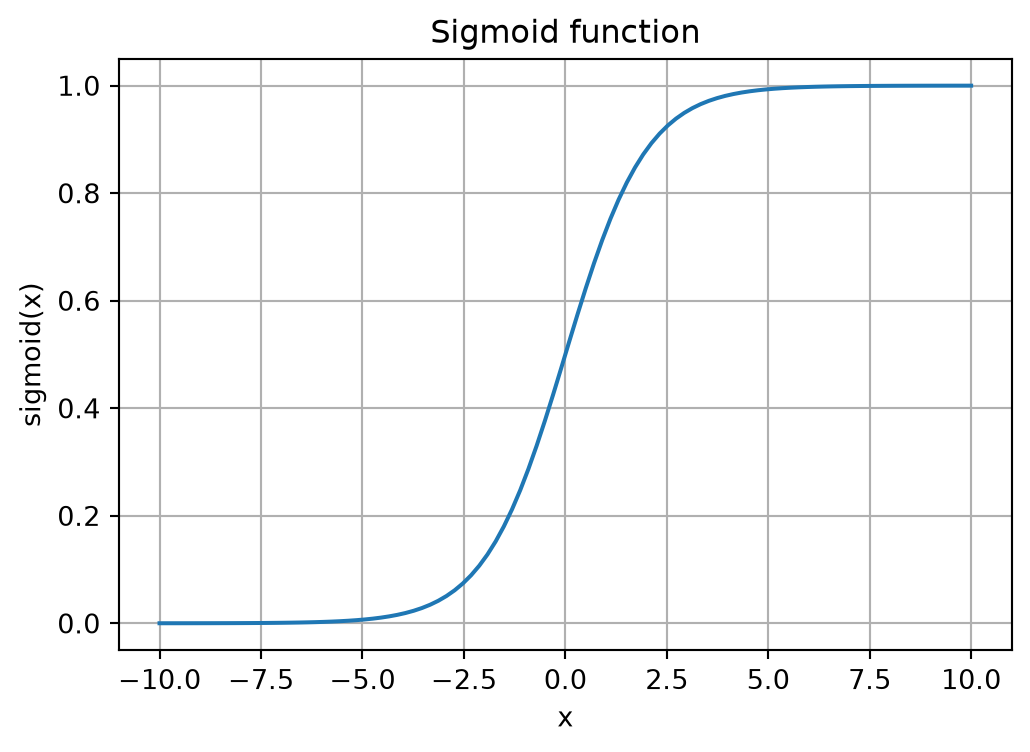
A single neuron with a sigmoid activation is essentially logistic regression!
Neural networks extend this by:
This allows neural networks to learn complex, non-linear decision boundaries.
An artificial neuron is loosely modeled on biological neurons:
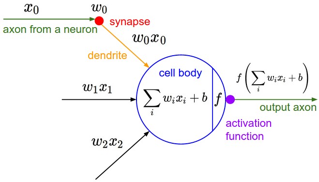
From cs231n
A neuron performs the following operation:
\[ \text{output} = f\left(\sum_{i=1}^n w_i x_i + b\right) \]
Where:
ReLU (Rectified Linear Unit) - most popular today: \[ \text{ReLU}(x) = \max(0, x) \]
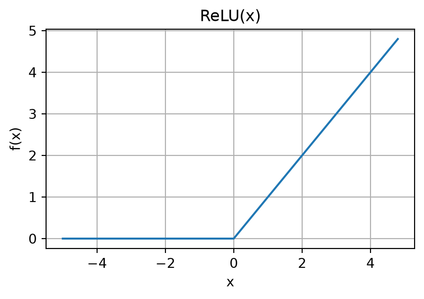
Why activation functions?
Answer: Without non-linearity, multiple layers collapse to a single linear transformation!
A Multi-Layer Perceptron stacks multiple layers of neurons:
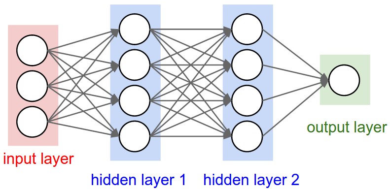
From cs231n

Key property: Every neuron in layer \(i\) connects to every neuron in layer \(i+1\).
This is also called a Fully Connected Network (FCN) or Dense Network.
For a network with \(K\) hidden layers:
\[ \begin{aligned} \mathbf{h}_1 &= f(\boldsymbol{\beta}_0 + \boldsymbol{\Omega}_0 \mathbf{x}) \\ \mathbf{h}_2 &= f(\boldsymbol{\beta}_1 + \boldsymbol{\Omega}_1 \mathbf{h}_1) \\ &\vdots \\ \mathbf{h}_K &= f(\boldsymbol{\beta}_{K-1} + \boldsymbol{\Omega}_{K-1} \mathbf{h}_{K-1}) \\ \mathbf{\hat{y}} &= \boldsymbol{\beta}_K + \boldsymbol{\Omega}_K \mathbf{h}_K \end{aligned} \]
Where:
Note: from here on \(\boldsymbol\beta_k\) is a bias vector, following the UDL textbook – not the regression coefficients \(\boldsymbol\beta\) of the linear-regression slide.
Training means finding weights that minimize a loss function:
For regression (e.g., predicting house prices): \[ L = \frac{1}{N}\sum_{i=1}^N (\hat{y}_i - y_i)^2 \quad \text{(Mean Squared Error)} \]
For classification (e.g., digit recognition): \[ L = -\frac{1}{N}\sum_{i=1}^N \sum_{c=1}^C y_{ic} \log(\hat{y}_{ic}) \quad \text{(Cross-Entropy)} \]
For classification the output layer is followed by a softmax (a sigmoid when \(C = 2\)), so the \(\hat y_{ic}\) are probabilities.
Goal: Find parameters \(\theta = \{\boldsymbol{\Omega}_k, \boldsymbol{\beta}_k\}\) that minimize \(L\). We write \(\theta\) for all the parameters, and \(\mathbf{w}\) when an argument applies to any collection of them.
The loss function creates a surface over the parameter space:
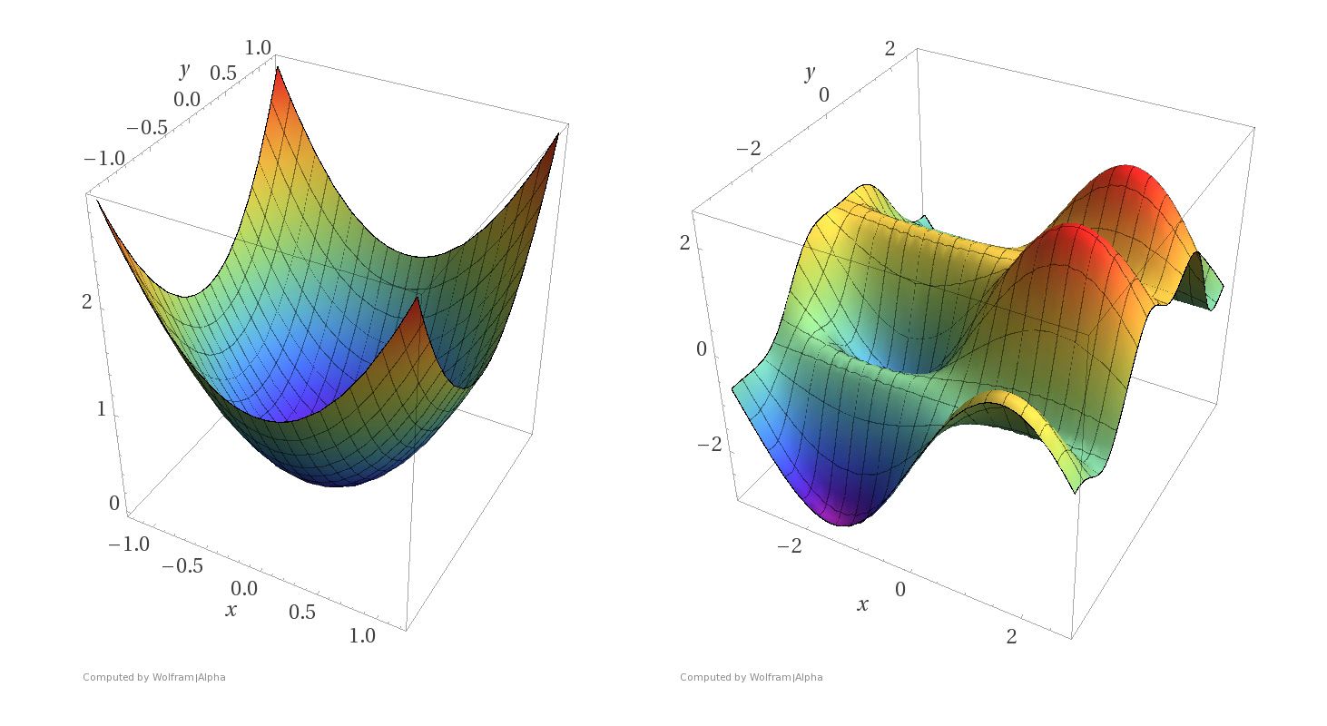
For neural networks, we can’t solve analytically—we need gradient descent!
Imagine you’re lost in foggy mountains and want to reach the valley:

What would you do?
This is gradient descent!
For a function \(L(\mathbf{w})\) of \(p\) parameters, \(\mathbf{w} = (w_1, \ldots, w_p)\), the gradient is:
\[ \nabla_\mathbf{w} L(\mathbf{w}) = \begin{bmatrix} \frac{\partial L}{\partial w_1}\\ \frac{\partial L}{\partial w_2}\\ \vdots \\ \frac{\partial L}{\partial w_p} \end{bmatrix} \]
Start with random weights \(\mathbf{w}^{(0)}\), then iterate:
\[ \mathbf{w}^{(t+1)} = \mathbf{w}^{(t)} - \eta \nabla_\mathbf{w} L(\mathbf{w}^{(t)}) \]
Where:
Stop when:
The first rule is what Lecture 17’s early_stopping will mean.
On \(L(w) = 3w^2 - 4w + 5\) (minimum at \(w = 2/3\)) the gradient is \(6w - 4\), so each step multiplies the distance to the minimum by \((1 - 6\eta)\). Eight steps from \(w = -3\) (black square):
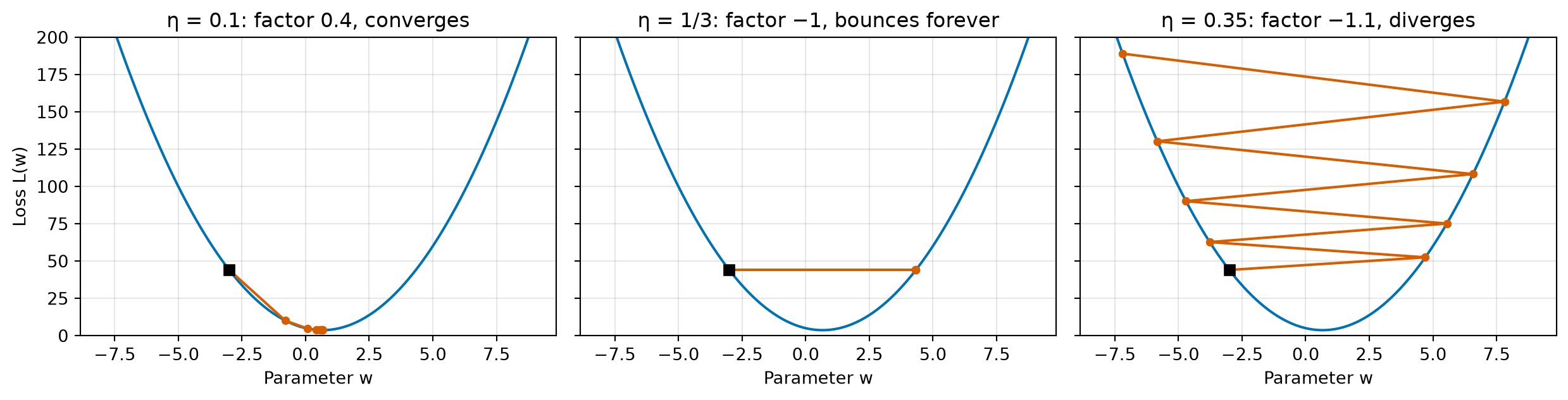
Too small a rate is merely slow; once \(|1 - 6\eta| > 1\), i.e. \(\eta > 1/3\), every step overshoots by more than it started with and the loss grows.
Linear regression’s loss \(\tfrac12\Vert\mathbf{y} - X\boldsymbol\beta\Vert^2\) on 10 points (Module M11’s example), as contours over the two parameters:
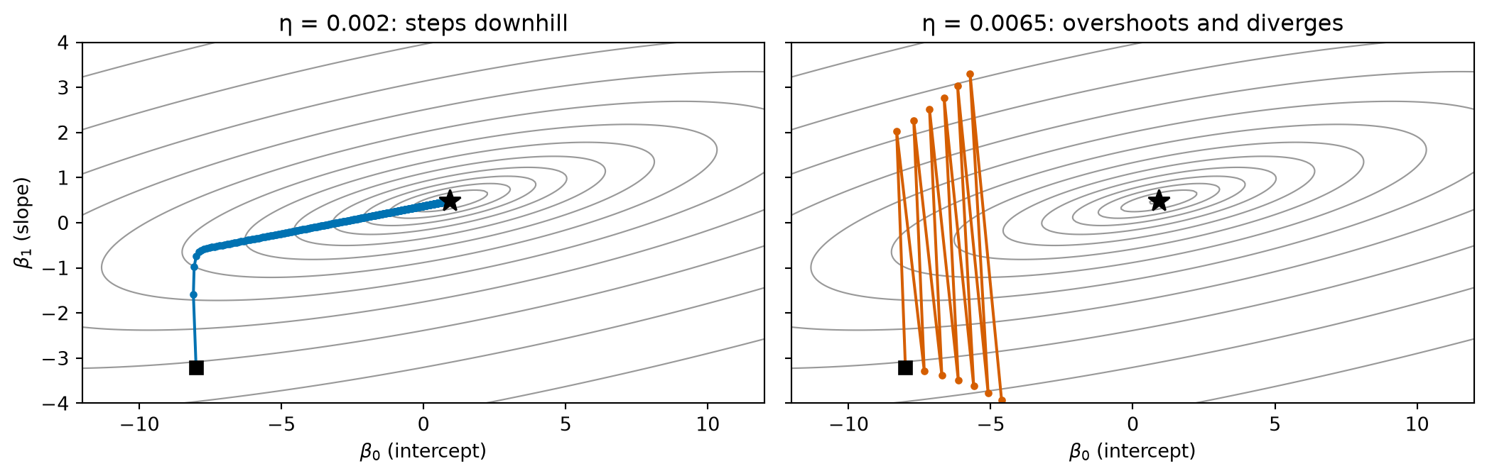
Square: start; star: least-squares solution. A convex surface has one basin, so a small step gets there (slowly, along the shallow valley); at \(\eta = 0.0065\) each step overshoots across the steep direction.
Gradient descent needs \(\nabla_\theta L\) – the partial derivative of the loss with respect to every weight and bias in the network.
But \(L\) is a deeply nested composition:
\[ L = \ell\big(\,\boldsymbol{\beta}_K + \boldsymbol{\Omega}_K\, f(\boldsymbol{\beta}_{K-1} + \boldsymbol{\Omega}_{K-1}\, f(\cdots f(\boldsymbol{\beta}_0 + \boldsymbol{\Omega}_0 \mathbf{x})\cdots))\,,\ y\big) \]
That something is backpropagation: the chain rule, organized on a computation graph.
The way we are going to differentiate more complex functions is to first build a “computation graph.”
We’ll see that we can “propagate backwards” through the graph to calculate the gradients of the loss function with respect to the parameters.
It’s a scalable approach employed by TensorFlow and PyTorch, and in fact we’ll follow the PyTorch interface definition.
This section is a condensed version of Module M12: the full Value framework, which builds the class step by step and turns it into a training framework.
Value ClassWe will
class called Value,This is similar to how PyTorch defines its Tensor class.
The class on the next slide has four parts: the stored number (data), a gradient slot (grad), a record of how the node was made (_prev, _op), and the operations +, *, relu() and loss(). Each operation returns a new Value that remembers its operands – that is how the graph builds itself.
class Value:

    def __init__(self, data, _children=(), _op='', label=''):
        self.data = data
        self.grad = 0.0               # dL/d(this node), filled in by backprop
        self._prev = set(_children)   # the operand nodes
        self._op = _op                # the operation that created this node
        self.label = label            # a name, for drawing

    def __repr__(self):
        return f"Value(data={self.data})"

    def __add__(self, other):         # self + other
        other = other if isinstance(other, Value) else Value(other)
        return Value(self.data + other.data, (self, other), '+')

    def __mul__(self, other):         # self * other
        other = other if isinstance(other, Value) else Value(other)
        return Value(self.data * other.data, (self, other), '*')

    def relu(self):
        return Value(max(0.0, self.data), (self,), 'ReLU')

    def loss(self, y):                # squared-error loss 1/2 (self - y)^2
return Value(0.5 * (self.data - y) ** 2, (self,), '½(ŷ−y)²')Value ClassWhen Python evaluates a * b, it calls a.__mul__(b); a * b + c then calls __add__ on the temporary product.
a = Value(4.0, label='a')
b = Value(-3.0, label='b')
c = Value(8.0, label='c')

d = a*b ; d.label = 'd'
e = d + c ; e.label = 'e'
eValue(data=-4.0)Each result remembers its operands and the operation that created it:
e._prev, e._op({Value(data=-12.0), Value(data=8.0)}, '+')We now have enough information stored to visualize the graph. Two helper functions walk the graph to collect all nodes and edges (trace) and draw them as a directed graph (draw_dot).
trace() and draw_dot()from graphviz import Digraph
def trace(root):
# builds a set of all nodes and set of all edges in a graph
nodes, edges = set(), set()
def build(v):
if v not in nodes:
nodes.add(v)
for child in v._prev:
edges.add((child, v))
build(child)
build(root)
return nodes, edges
def draw_dot(root):
dot = Digraph(format='svg',
graph_attr={'rankdir': 'LR', 'ranksep': '0.3', 'nodesep': '0.15',
'size': '11,4'},
node_attr={'fontsize': '20'})
nodes, edges = trace(root)
for n in nodes:
uid = str(id(n))
# one box per Value, with its name, data and grad stacked
# (+ 0.0 turns a negative zero into a plain 0)
dot.node(name=uid, shape='record',
label="%s | data %.4g | grad %.4g" % (n.label, n.data + 0.0, n.grad + 0.0))
if n._op:
# an operator node, feeding the Value it produced
dot.node(name=uid + n._op, label=n._op)
dot.edge(uid + n._op, uid)
for n1, n2 in edges:
dot.edge(str(id(n1)), str(id(n2)) + n2._op)
return dotLet’s build a small three-stage graph, ending in a node we’ll call L.
a = Value(4.0, label='a')
b = Value(-3.0, label='b')
c = Value(8.0, label='c')

d = a*b; d.label = 'd'
e = d + c; e.label = 'e'
f = Value(2.0, label='f')

L = e*f; L.label = 'L'
draw_dot(L)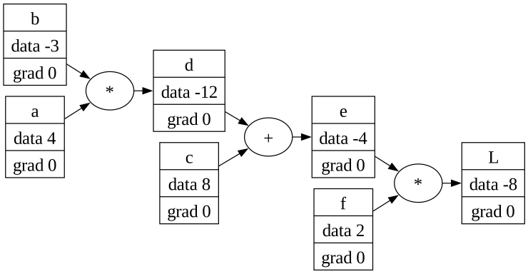
Every Value becomes a box; the operators are drawn as small nodes too. Computing the data values left-to-right is the forward pass.
We have placeholders for the gradients, but they are currently all zero.
Before we automate backpropagation, let’s calculate the gradients by hand to understand the procedure.
For the output node \(L\), we trivially have \(\frac{dL}{dL} = 1\):
\[ \frac{dL}{dL} = \lim_{h \rightarrow 0} \frac{ (L+h) - L }{h} = \frac{h}{h} = 1 \]
L.grad = 1.0Going backwards one step, \(L = e \times f\), so
\[ \frac{\partial{L}}{\partial{e}} = \frac{\partial}{\partial{e}} (e\times f) = f, \qquad \frac{\partial{L}}{\partial{f}} = \frac{\partial}{\partial{f}} (e\times f) = e. \]
So we just assign the gradient to the value of the other operand.
For products, the partial derivative w.r.t. one operand is simply the other operand.
We needed the node values e.data and f.data to compute these gradients. All the node values come from the forward pass – so the forward pass must run first.
e.grad = f.data
f.grad = e.data
draw_dot(L)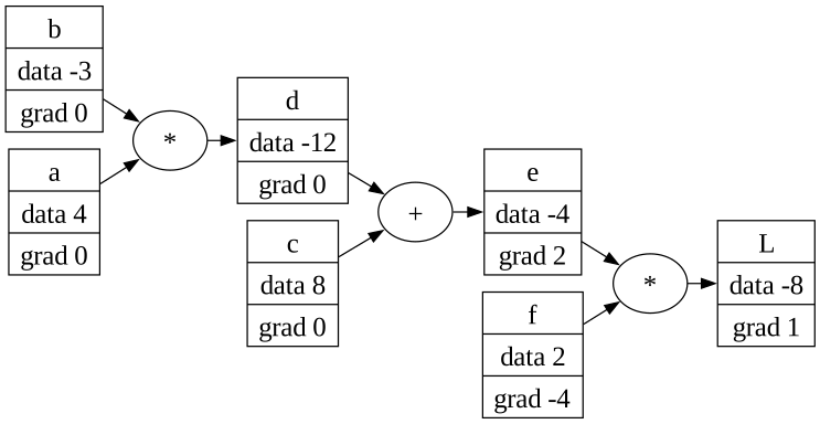
Sanity check: f.grad says \(L\) should change by e.data \(= -4\) for a unit change in \(f\). wiggle rebuilds the graph with one input raised by \(h\) and reports the slope \(\big(L(\text{input} + h) - L(\text{input})\big)/h\).
def wiggle(build, params, var, h=1.0):
    L0 = build(**params).data
    L1 = build(**{**params, var: params[var] + h}).data
    print(f"L: {L0:g} -> {L1:g} when {var} goes up by {h:g};  slope = {(L1 - L0) / h:g}")

def toy_graph(a, b, c, f):
    return (Value(a) * Value(b) + Value(c)) * Value(f)

toy = dict(a=4.0, b=-3.0, c=8.0, f=2.0)
wiggle(toy_graph, toy, 'f')
L: -8 -> -12 when f goes up by 1; slope = -4Now we want \(\frac{\partial{L}}{\partial{c}}\) – how much \(L\) varies if we vary \(c\).
Looking at the graph, \(c\) influences \(e\) and \(e\) influences \(L\):
\[ c \rightarrow e \rightarrow L. \]
We have \(e = d + c\), so the local derivative is
\[ \frac{\partial{e}}{\partial{c}} = \frac{\partial{}}{\partial{c}} (d + c) = 1. \]
For addition, the partial derivative w.r.t. either operand is 1.
We know \(\partial{L}/\partial{e}\) and we know \(\partial{e}/\partial{c}\). How do we get \(\partial{L}/\partial{c}\)?
If a variable \(L\) depends on the variable \(e\), which itself depends on the variable \(c\), then \(L\) depends on \(c\) as well, via the intermediate variable \(e\), and
\[ \frac{\partial L}{\partial c} = \frac{\partial L}{\partial e} \cdot \frac{\partial e}{\partial c}. \]
More precisely, noting where each derivative is evaluated:
\[ \left.\frac{\partial L}{\partial c}\right|_{c} = \left.\frac{\partial L}{\partial e}\right|_{e(c)}\cdot \left. \frac{\partial e}{\partial c}\right|_{c}. \]
We evaluate the derivatives at the specific values of the variables that we calculated in the forward pass.
Since \(\partial e/\partial c = 1\),
\[ \frac{\partial L}{\partial c} = \frac{\partial L}{\partial e} \cdot \frac{\partial{e}}{\partial{c}} = \frac{\partial L}{\partial e} \cdot 1, \]
and identically for \(d\).
With the addition operator, we just route the parent gradient to the child.
d.grad = e.grad
c.grad = e.grad
draw_dot(L)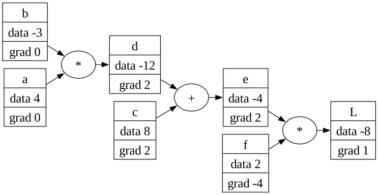
One more step. We have \(\frac{\partial{L}}{\partial{d}}\) and want \(\frac{\partial{L}}{\partial{a}}\) and \(\frac{\partial{L}}{\partial{b}}\).
Since \(d = a \cdot b\), the local derivatives are \(\partial d/\partial b = a\) and \(\partial d/\partial a = b\), so by the chain rule
\[ \frac{\partial{L}}{\partial{b}} = \frac{\partial{L}}{\partial{d}} \cdot \frac{\partial{d}}{\partial{b}} = \frac{\partial{L}}{\partial{d}} \cdot a, \qquad \frac{\partial{L}}{\partial{a}} = \frac{\partial{L}}{\partial{d}} \cdot b. \]
Fully expanded, this is a chain of local derivatives all the way from \(L\) back to \(b\):
\[ \frac{\partial{L}}{\partial{b}} = \frac{\partial{L}}{\partial{e}} \cdot \frac{\partial{e}}{\partial{d}} \cdot \frac{\partial{d}}{\partial{b}}. \]
b.grad = a.data * d.grad
a.grad = b.data * d.grad
draw_dot(L)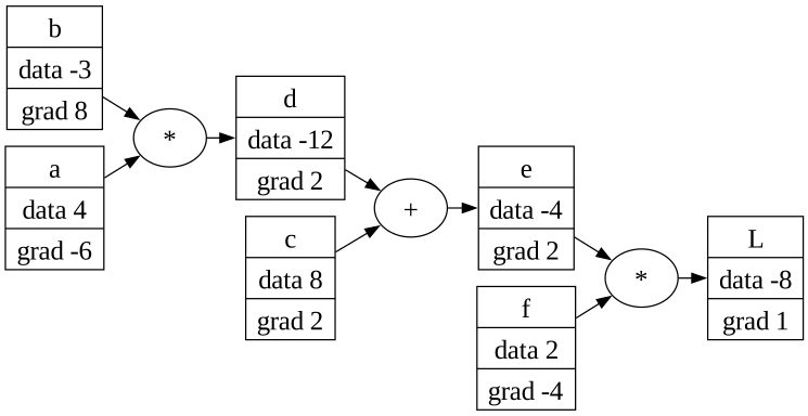
We’ve traversed all the way back to the inputs and calculated all the partial derivatives.
Check: b.grad \(= 8\), so raising \(b\) by \(1\) should raise \(L\) by \(8\).
wiggle(toy_graph, toy, 'b')L: -8 -> 0 when b goes up by 1; slope = 8data.L.grad = 1.+ node: pass the gradient through unchanged* node: multiply by the other operand’s valueReLU node: pass through if the input was \(> 0\), otherwise send \(0\)Every step is local – each node and edge is visited once, as in the forward pass – so the backward pass costs a small constant multiple of one forward pass, however many parameters there are. This is the essence of backpropagation.
The same recipe applies to a real neuron. Here is one with two inputs, two weights, a bias, and a ReLU:
# inputs x1, x2
x1 = Value(2.0, label='x1')
x2 = Value(0.0, label='x2')

# weights w1, w2
w1 = Value(-3.0, label='w1')
w2 = Value(1.0, label='w2')

# bias of the neuron
b = Value(7.0, label='b')

x1w1 = x1*w1; x1w1.label = 'x1*w1'
x2w2 = x2*w2; x2w2.label = 'x2*w2'

x1w1x2w2 = x1w1 + x2w2; x1w1x2w2.label = 'x1w1 + x2w2'
n = x1w1x2w2 + b; n.label = 'n'
o = n.relu(); o.label = 'o'
draw_dot(o)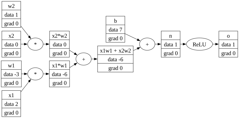
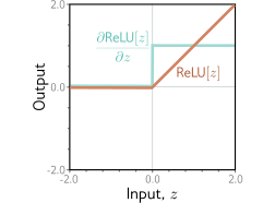
The only new operation is the ReLU. It is technically not differentiable at 0, but in practice we take the derivative to be \(0\) when the input is \(\le 0\) and \(1\) when it is \(> 0\).
o.grad = 1.0
n.grad = o.grad if n.data > 0 else 0.0   # ReLU: pass through if the input was positive
x1w1x2w2.grad = n.grad                    # '+' routes the gradient
b.grad = n.grad
x1w1.grad = x1w1x2w2.grad
x2w2.grad = x1w1x2w2.grad
w1.grad = x1.data * x1w1.grad             # '*' multiplies by the other operand
w2.grad = x2.data * x2w2.grad
draw_dot(o)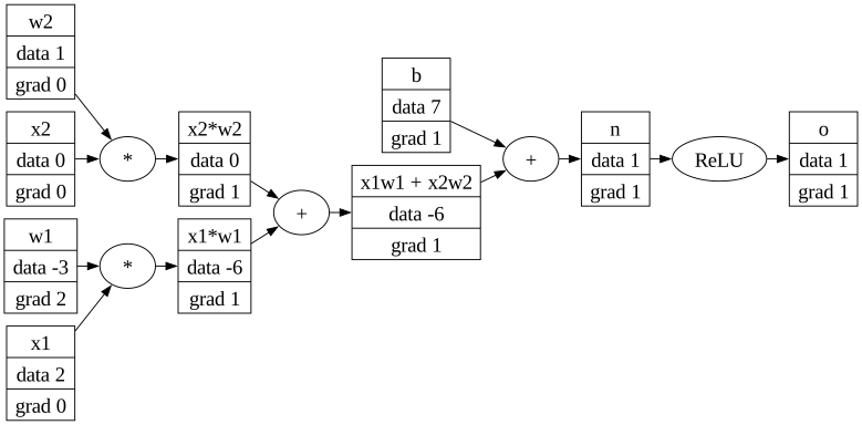
Note w2.grad \(= 0\) because \(x_2 = 0\): this weight has no influence on the output for this input. That is the * rule at work – a zero input to a product.
Real training puts a loss on top. Here is the smallest network with everything: one input, one hidden ReLU unit, one output, and the squared-error loss.
\[ z_1 = w_1 x + b_1,\qquad h = \mathrm{ReLU}(z_1),\qquad \hat y = w_2 h + b_2,\qquad L = \tfrac12(\hat y - y)^2 \]
with \(w_1 = 1,\ b_1 = 0.5,\ w_2 = -2,\ b_2 = 1\) and one training example \(x = 1,\ y = 0\).
Forward pass by hand: \(z_1 = 1\cdot 1 + 0.5 = 1.5\), \(\ h = 1.5\), \(\ \hat y = -2\cdot 1.5 + 1 = -2\), \(\ L = \tfrac12(-2 - 0)^2 = 2\).
The same network as a Value graph:
from types import SimpleNamespace

def two_layer(w1, b1, w2, b2, x, y):
    g = SimpleNamespace(y=y)
    g.x, g.w1, g.b1 = Value(x, label='x'), Value(w1, label='w1'), Value(b1, label='b1')
    g.w2, g.b2 = Value(w2, label='w2'), Value(b2, label='b2')
    g.w1x = g.w1 * g.x;     g.w1x.label = 'w1*x'
    g.z1 = g.w1x + g.b1;    g.z1.label = 'z1'
    g.h = g.z1.relu();      g.h.label = 'h'
    g.w2h = g.w2 * g.h;     g.w2h.label = 'w2*h'
    g.yhat = g.w2h + g.b2;  g.yhat.label = 'yhat'
    g.L = g.yhat.loss(y);   g.L.label = 'L'
    return g

params = dict(w1=1.0, b1=0.5, w2=-2.0, b2=1.0)
net = two_layer(**params, x=1.0, y=0.0)
draw_dot(net.L)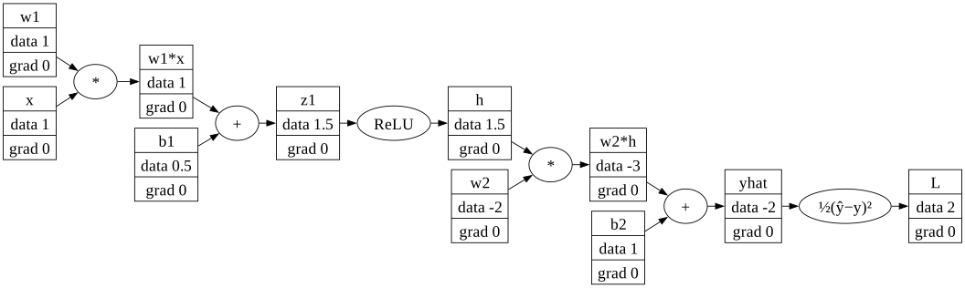
The recipe, node by node from the top. The loss node’s local derivative is \(\partial L/\partial\hat y = \hat y - y\):
def backward_by_hand(g):
    g.L.grad = 1.0
    g.yhat.grad = (g.yhat.data - g.y) * g.L.grad      # loss node: send yhat - y
    g.w2h.grad = g.yhat.grad                          # '+' routes
    g.b2.grad = g.yhat.grad
    g.w2.grad = g.h.data * g.w2h.grad                 # '*' multiplies by the other operand
    g.h.grad = g.w2.data * g.w2h.grad
    g.z1.grad = g.h.grad if g.z1.data > 0 else 0.0    # ReLU gates
    g.w1x.grad = g.z1.grad                            # '+' routes
    g.b1.grad = g.z1.grad
    g.w1.grad = g.x.data * g.w1x.grad                 # '*' again
    g.x.grad = g.w1.data * g.w1x.grad                 # (inputs get one too; unused)

backward_by_hand(net)
draw_dot(net.L)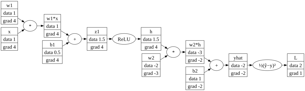
Reading the numbers off the graph, top to bottom:
+ routes it: \(\partial L/\partial b_2 = -2\)* swaps: \(\partial L/\partial w_2 = h \cdot (-2) = 1.5 \cdot (-2) = -3\), and \(\partial L/\partial h = w_2 \cdot (-2) = (-2)(-2) = 4\)+ routes: \(\partial L/\partial b_1 = 4\); * swaps: \(\partial L/\partial w_1 = x \cdot 4 = 4\)Written as one product of local derivatives, from the loss back to the first weight:
\[ \frac{\partial L}{\partial w_1} = \underbrace{\frac{\partial L}{\partial \hat y}}_{\hat y - y} \cdot \underbrace{\frac{\partial \hat y}{\partial h}}_{w_2} \cdot \underbrace{\frac{\partial h}{\partial z_1}}_{\text{ReLU}'(z_1)} \cdot \underbrace{\frac{\partial z_1}{\partial w_1}}_{x} = (-2)(-2)(1)(1) = 4. \]
So raising \(w_1\) by \(0.01\) should raise the loss by about \(4 \times 0.01 = 0.04\). Check:
def net_loss(**p):
    return two_layer(**p).L

wiggle(net_loss, dict(**params, x=1.0, y=0.0), 'w1', h=0.01)
L: 2 -> 2.0402 when w1 goes up by 0.01; slope = 4.02The finite difference, \(4.02\), agrees with backprop’s \(4\) (the extra \(0.02\) is the curvature a step of \(h = 0.01\) picks up).
Now use the gradients. One step of gradient descent with \(\eta = 0.05\) on each parameter leaf, \(w \leftarrow w - \eta\,\partial L/\partial w\), then a fresh forward pass:
eta = 0.05
new_params = {k: v - eta * getattr(net, k).grad for k, v in params.items()}
new_net = two_layer(**new_params, x=1.0, y=0.0)

print({k: round(v, 3) for k, v in new_params.items()})
print(f"yhat: {net.yhat.data:g} -> {new_net.yhat.data:g}    "
      f"loss: {net.L.data:g} -> {new_net.L.data:.4g}")
{'w1': 0.8, 'b1': 0.3, 'w2': -1.85, 'b2': 1.1}
yhat: -2 -> -0.935 loss: 2 -> 0.4371Every parameter moved against its gradient: \(w_1 = 1 - 0.05(4) = 0.8\), \(b_1 = 0.5 - 0.05(4) = 0.3\), \(w_2 = -2 - 0.05(-3) = -1.85\), \(b_2 = 1 - 0.05(-2) = 1.1\). The prediction moved from \(-2\) toward the target \(0\), and the loss fell from \(2\) to \(0.437\). That is one iteration of training.
Same parameters, but flip the sign of the input: \(x = -1\). Now \(z_1 = -1 + 0.5 = -0.5 < 0\), so \(h = 0\), \(\hat y = b_2 = 1\) and \(L = \tfrac12\).
dead = two_layer(**params, x=-1.0, y=0.0)
backward_by_hand(dead)
draw_dot(dead.L)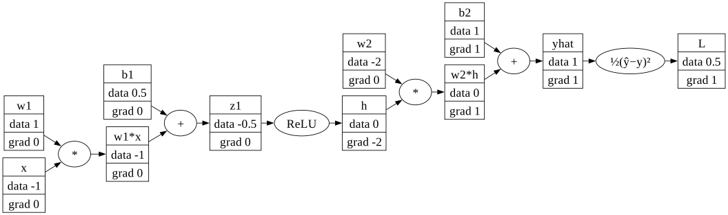
Two different zeros, from two different rules:
* rule, because \(w_2\)’s input \(h\) is \(0\) – the same mechanism as w2.grad \(= 0\) in the neuron example.If every training example put the unit in this state, \(w_1\) and \(b_1\) would never change and the unit would output \(0\) forever: a dead (or “dying”) ReLU. A too-large step can push a unit into this state, which is one reason the learning rate and initialisation matter, and why variants such as leaky ReLU exist.
In Module M12 we finish the job: add a backward() method to Value that walks the graph automatically, handle nodes used more than once (gradients accumulate), assemble neurons into layers and an MLP, and write the training loop. In Neural Networks II we let scikit-learn do all of that for us.
Backprop gives us the gradient of the loss for one sample, \(\nabla_\mathbf{w} \ell_i(\mathbf{w})\). How many samples should we run it on before taking a step?
Full Batch Gradient Descent: Compute gradient using ALL training samples:
\[ \nabla_\mathbf{w} L = \frac{1}{N}\sum_{i=1}^N \nabla_\mathbf{w} \ell_i(\mathbf{w}) \]
Problems:
Stochastic Gradient Descent: Historically meant using ONE random sample at a time:
\[ \mathbf{w}^{(t+1)} = \mathbf{w}^{(t)} - \eta \nabla_\mathbf{w} \ell_i(\mathbf{w}^{(t)}) \]
Advantages:
Disadvantage:
Mini-Batch GD: Best of both worlds—use a small batch of samples:
\[ \nabla_\mathbf{w} L \approx \frac{1}{B}\sum_{i \in \text{batch}} \nabla_\mathbf{w} \ell_i(\mathbf{w}) \]
Typical batch sizes: 32, 64, 128, 256
Advantages:
This is what most modern neural network training uses!
Linear regression, \(N = 1000\) synthetic points, \(\eta = 0.05\) for every batch size. Vertical axis: training MSE on all \(N\) points minus the best achievable (least squares).
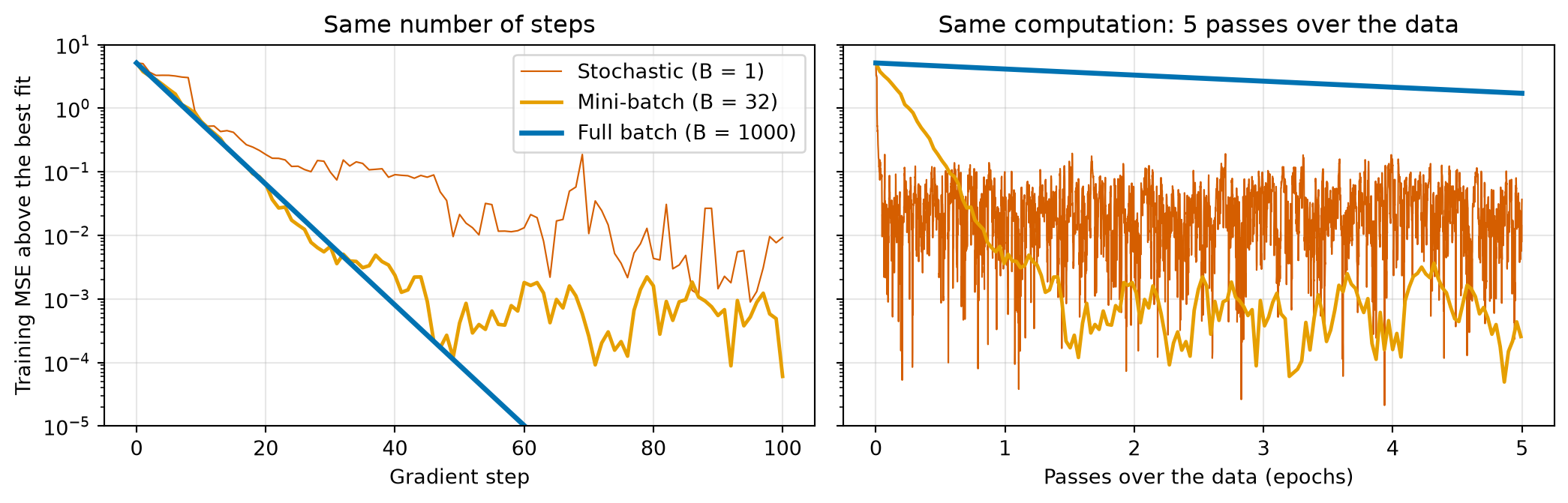
Per step (left) the full batch wins; mini-batch and SGD stall at a noise floor. Per unit of computation (right) the full batch has taken only 5 steps while mini-batch reaches its floor in about one pass.
+ routes, * swaps, ReLU gates, the loss node sends \(\hat y - y\)In Neural Networks II we switch to practice: MLPClassifier and MLPRegressor in scikit-learn, MNIST and California housing, hyperparameters, preprocessing, and how to recognize and fix training that isn’t working.
Full treatments of today’s topics in the course notes:
Value framework: the class built step by step, automatic backward(), gradient accumulation, and a complete training loopAdditional resources: