Recap: Soft Clustering with Gaussian Mixture Models
DS701 Session 7 — Mon Sep 28, 2026


Today’s plan
- 5 min — knowledge-check review
- 20 min — highlights and Q&A (answer or pass — answering always earns credit)
- 60 min — in-class activity (small groups)
- wrap-up and cold-call check-ins
Knowledge-Check Review
KC 1: The generative story
A Gaussian mixture model is a generative story. Describe, in two steps, how the model says a single data point \(x_i\) is produced, and write down the resulting density \(p(x_i \mid \theta)\). What are the parameters \(\theta\)?
Show answer
Answer:
- Pick a component \(k \in \{1, \dots, K\}\) with probability \(\pi_k\) (the mixing weights, \(\sum_k \pi_k = 1\)).
- Draw \(x_i \sim \mathcal{N}(\mu_k, \Sigma_k)\) from that component’s Gaussian.
Averaging over the hidden choice:
\[ p(x_i \mid \theta) = \sum_{k=1}^{K} \pi_k\, \mathcal{N}(x_i \mid \mu_k, \Sigma_k), \qquad \theta = \{\pi_k, \mu_k, \Sigma_k\}_{k=1}^{K}. \]
A weighted sum of \(K\) bell curves; one weight, one mean, one covariance per component.
KC 2: Why EM?
In lecture 05 we found the MLE for a single Gaussian by taking the log-likelihood, differentiating, and solving in closed form (sample mean, sample variance). Why does the same approach not work for a mixture, and how do the two EM steps get around it? Say specifically what the E-step and the M-step each compute.
Show answer
Answer: for a mixture each point’s density is a sum over components, so
\[ \ell(\theta) = \sum_{i=1}^{n} \log \Big( \sum_{k=1}^{K} \pi_k\, \mathcal{N}(x_i \mid \mu_k, \Sigma_k) \Big) \]
has a sum inside the log: derivatives couple every parameter, no closed form. If we knew which component produced each point it would split into \(K\) ordinary Gaussian MLEs — but we don’t.
- E-step — with the current \(\theta\), compute responsibilities \(\gamma_{ik} = P(z_i = k \mid x_i)\) by Bayes’ rule (soft assignments; each row sums to 1).
- M-step — treat the \(\gamma_{ik}\) as fractional memberships and re-estimate \(\mu_k, \Sigma_k, \pi_k\) with the weighted lecture-05 formulas.
Each round can only increase \(\ell\) — so it converges, to a local maximum.
KC 3: “Just \(k\)-means with probabilities”?
A classmate says “a GMM is just \(k\)-means with probabilities attached.” Name two ways that description is incomplete, and give one dataset the lecture showed where the difference visibly matters.
Show answer
Answer: any two of
- Soft assignment is used inside the algorithm — the M-step averages over all points, weighted, so a 50/50 point pulls on two components at once.
- Cluster shape — a covariance per component (full / tied / diag / spherical, chosen explicitly): elongated, rotated, differently sized clusters. \(k\)-means implicitly assumes round, equal-radius clusters.
- Explicit generative assumption — “the data came from a mixture of Gaussians”, which we can inspect and swap; \(k\)-means merely declared an objective.
- It is a density: we can score new points and compare models.
Dataset: the thin diagonal cluster next to a round blob — \(k\)-means hands the tip of the thin cluster to the blob; the GMM recovers both. Or the overlapping clusters, where a hard label is not even the honest answer.
Highlights
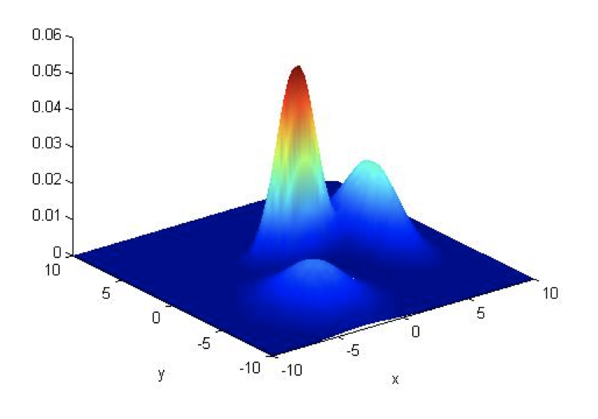
The model is a recipe for making data
For each of the \(n\) points, independently:
- roll a \(K\)-sided die with face probabilities \(\pi_1, \dots, \pi_K\) — that is the latent label \(z_i\);
- draw \(x_i\) from the Gaussian for that face, \(\mathcal{N}(\mu_{z_i}, \Sigma_{z_i})\).
Forget the die roll and you get the mixture density \[ p(x \mid \theta) = \sum_{k=1}^{K} \pi_k\, \mathcal{N}(x \mid \mu_k, \Sigma_k). \]
Clustering = running the recipe backwards: given only the \(x_i\), recover \(\theta\) and say how each point was probably rolled.
E-step: Bayes’ rule, one point at a time
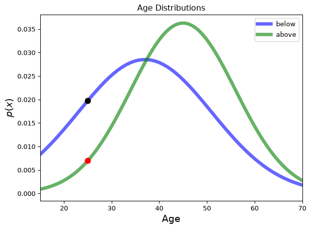
Age 25 in the income example. Black dot: density under below; red dot: density under above.
\[ P(\text{above} \mid 25) = \frac{\text{red}\cdot P(\text{above})}{\text{red}\cdot P(\text{above}) + \text{black}\cdot P(\text{below})} \]
Same thing for every point \(i\) and component \(k\): \[ \gamma_{ik} = \frac{\pi_k\, \mathcal{N}(x_i \mid \mu_k, \Sigma_k)}{\sum_{j} \pi_j\, \mathcal{N}(x_i \mid \mu_j, \Sigma_j)} \]
prior \(\pi_k\), likelihood \(\mathcal{N}(\cdot)\), evidence = the mixture density. Rows sum to 1.
M-step: lecture 05, weighted
One Gaussian (lecture 05) — the MLE: \[ \bar\mu = \frac{1}{N}\sum_{i} x_i, \qquad \bar\sigma^2 = \frac{1}{N}\sum_{i} (x_i - \bar\mu)^2 \]
Component \(k\) of a mixture — with \(N_k = \sum_i \gamma_{ik}\):
\[ \mu_k = \frac{1}{N_k}\sum_i \gamma_{ik}\, x_i, \quad \Sigma_k = \frac{1}{N_k}\sum_i \gamma_{ik}\,(x_i-\mu_k)(x_i-\mu_k)^{\!T}, \quad \pi_k = \frac{N_k}{n} \]
- Every point contributes to every component, weighted by how responsible that component is for it.
- \(N_k\) is an effective count — usually not an integer.
- Set all \(\gamma_{ik} \in \{0, 1\}\) and the formulas collapse to per-cluster means: the \(k\)-means update.
- That is the whole trick: pretend the soft assignments are true memberships and do MLE.
Why iterate at all — and what you get for it
- Direct maximization: \(\sum_i \log(\sum_k \cdots)\) — the sum inside the log couples every parameter. No closed form.
- Chicken 🐓 and egg 🥚: labels ⇒ easy parameters; parameters ⇒ easy labels; we have neither.
- EM: guess parameters → E-step (soft labels) → M-step (weighted MLE) → repeat.
- Guaranteed: the log-likelihood never decreases, so it converges.
- Not guaranteed: the global maximum. Local optimum, depends on the start — like \(k\)-means, NP-hard in general. Initialize with \(k\)-means; restart several times.
- Stop when \(|\ell^{(t)} - \ell^{(t-1)}| < \text{tol}\), or the parameters stop moving, or
max_iter.
GMM vs. \(k\)-means, side by side
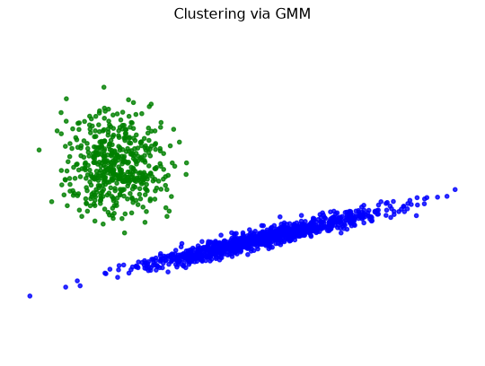
covariance_type="full"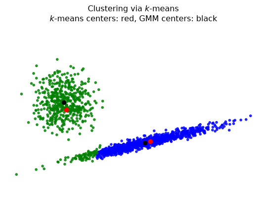
- Same two-phase loop; soft vs. hard assignment is the practical difference (“soft \(k\)-means”).
- The GMM’s assumption is explicit — a mixture of Gaussians — so it can be inspected, tightened, or swapped. \(k\)-means only declared an objective.
- Here the explicit covariance is what saves the thin cluster’s tip: nearest-center distance hands it to the blob.
Choosing how much shape to allow
covariance_type is where the assumption becomes a dial (\(K\) components in \(d\) dimensions):
| type | each \(\Sigma_k\) is | shape | covariance parameters |
|---|---|---|---|
spherical |
\(\sigma_k^2 I\) | circle, own radius | \(K\) |
diag |
diagonal | axis-aligned ellipse | \(Kd\) |
tied |
one shared \(\Sigma\) | same ellipse everywhere | \(\sim d^2\) |
full |
its own \(\Sigma_k\) | any ellipse | \(\sim Kd^2\) |
More parameters need more data per cluster; fewer parameters is a stronger claim about the world. Today’s activity makes you see the difference — and see what a 50/50 responsibility looks like next to a \(k\)-means boundary.
EM Expainer Video
Going deeper
Full lecture notes: Soft Clustering with Gaussian Mixture Models
- Soft Clustering — the income/age example and conditional probability
- MLE in One Slide — the lecture-05 callback the M-step is built on
- The Gaussian Mixture Model — the generative story and the mixture density
- The Log-Likelihood Challenge — the sum inside the log
- E-Step and M-Step — the two updates
- Initialization and Iteration and Convergence
- k-means vs GMMs — soft vs. hard, explicit vs. implicit assumptions
- How many parameters are estimated? —
full/tied/diag/spherical - EM Explainer Video
- Appendices: MLE derivation, complete-data likelihood, deriving the E-step, deriving the M-step
- Next up: generalization — train/test discipline and overfitting (07).
In-Class Activity
Activity: EM by hand, then soft vs. hard — visualized
Goal: the lecture showed EM running as three short functions — now write them yourself, on a new 1-D two-component mixture; iterate while watching the log-likelihood climb; check against sklearn.mixture.GaussianMixture — then go to 2-D: responsibilities as color intensity next to \(k\)-means’ straight boundaries, the four covariance types as fitted ellipses, and one point the GMM calls 50/50.
- Work in groups of 2–3.
- Parts marked (autograded) are submitted to Gradescope; the rest is participation.
- Staff will circulate — be ready to explain any part of your work.
- Dependencies:
numpy,scipy,matplotlib,scikit-learnonly.


The activity notebook goes live on the day of the lecture. Colab is optional — you can also open it on GitHub and run it locally.