Recap: Causal Graphs and Estimating Effects
DS701 Session 18 — Wed Nov 4, 2026


Today’s plan
- 5 min — knowledge-check review
- 20 min — highlights and Q&A (answer or pass — answering always earns credit)
- 60 min — in-class activity (small groups)
- wrap-up and cold-call check-ins
Knowledge-Check Review
KC 1: Three building blocks
Name the three elementary structures every path in a causal DAG is built from, and for each say (i) what the middle node is called and (ii) whether the path through it is open or blocked by default, and what happens when you condition on that middle node.
KC 2: “Controlling for more can only help”
In the tutoring example, \(X\) = tutoring and \(Y\) = final grade, with \(\text{GPA}_{\text{prior}} \to X\), \(\text{GPA}_{\text{prior}} \to Y\), \(X \to \text{Hours} \to Y\) and \(X \to \text{HonorRoll} \leftarrow Y\). A colleague argues that adjusting for \(\{\text{GPA}_{\text{prior}}, \text{Hours}, \text{HonorRoll}\}\) must be at least as good* as adjusting for \(\{\text{GPA}_{\text{prior}}\}\) alone, “because controlling for more can only help.” Using the backdoor procedure, explain why the colleague is wrong about the total effect of tutoring — say what each of Hours and HonorRoll does to the estimate.*
KC 3: When the confounder is not in the data
Lecture I showed that randomization removes selection bias; this lecture showed that adjusting for a valid backdoor set does the same job with observational data. Suppose you believe there is a confounder you cannot measure (e.g. “motivation” driving both who takes a training program and later earnings). Explain in a sentence why regression adjustment cannot fix this, then name one of the three natural-experiment designs from the lecture, say in a sentence what “as good as random” variation it exploits, and state the key assumption it relies on instead.
Highlights
The graph is your assumptions, not the data’s
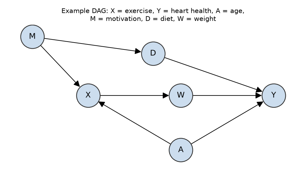
- Node = variable; arrow \(A \to X\) = “\(A\) is a direct cause of \(X\)” (\(A\) parent, \(X\) child).
- Directed path = follow the arrows: \(X \to W \to Y\). Nodes reachable this way are \(X\)’s descendants (\(W, Y\)).
- Acyclic: nothing is its own ancestor — cause precedes effect. Hence DAG.
- Path (undirected) = any chain of arrows, direction ignored: \(X \leftarrow A \to Y\) counts too.
Effects flow along directed paths; spurious association along the others. Domain knowledge draws the graph — data cannot — but once drawn, it tells you exactly what to control for.
Every path is chains, forks and colliders
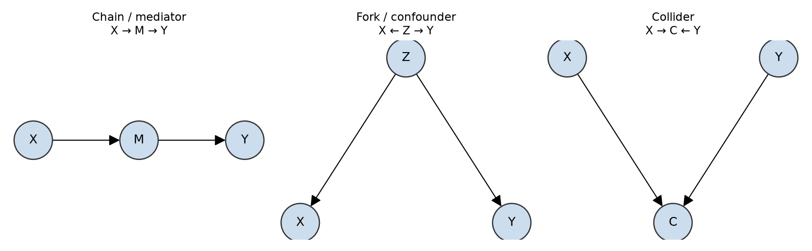
- Chain / fork node: open by default, blocked if you condition on it (adjust, stratify, put it in the regression).
- Collider node: blocked by default, opened if you condition on it — or on any of its descendants.
A path is blocked if at least one interior node is blocked; \(X\) and \(Y\) are independent given \(S\) when every path between them is blocked. Sanity check: \(X \leftarrow A \to Y\) is open (fork) — the ice-cream/temperature confounding of Lecture I; condition on \(A\) and it closes.
The golden rule: adjust for forks, not colliders or mediators
| structure | middle node | adjust for it? | why |
|---|---|---|---|
| fork \(X \leftarrow Z \to Y\) | confounder | yes | blocks the spurious backdoor path |
| chain \(X \to M \to Y\) | mediator | no* | it is the effect you want (overcontrol) |
| collider \(X \to C \leftarrow Y\) | collider | no! | conditioning creates association |
* unless you specifically want the direct, not the total, effect.
Talent and looks: independent by construction (corr \(\approx 0.00\)), yet among the famous corr \(\approx -0.55\) — restricting to the famous conditions on the collider talent \(\to\) famous \(\leftarrow\) looks. Selection is conditioning.
So “throw every variable into the regression” is wrong. Today’s stretch section makes you watch it go wrong on data you generated yourself.
The backdoor criterion is a procedure
A backdoor path starts with an arrow into \(X\) — confounding in graph language. \(S\) is a valid adjustment set if it blocks every backdoor path and contains no descendant of \(X\).
- List every path from \(X\) to \(Y\), ignoring direction.
- Set aside the causal paths (all arrows away from \(X\)) — never block these.
- The rest are backdoor paths: mark each open / blocked (forks & chains open, colliders closed).
- Choose \(S\) blocking every open backdoor — a fork or chain node on each — with no collider (or collider-descendant) and no descendant of \(X\).
- Report \(S\) — several may be valid; smallest is usually best.
Then — and only then — pick an estimator. Identification and estimation are separate decisions.
Worked example, five steps
\(A \to X,\ A \to Y,\ M \to X,\ M \to D,\ D \to Y,\ X \to W,\ W \to Y\)
- Paths: \(X \to W \to Y\); \(X \leftarrow A \to Y\); \(X \leftarrow M \to D \to Y\).
- Causal: \(X \to W \to Y\) — leave \(W\) alone.
- Backdoors: \(X \leftarrow A \to Y\) open (fork at \(A\)); \(X \leftarrow M \to D \to Y\) open (fork at \(M\), chain at \(D\)). No colliders.
- Block the first with \(A\); the second with \(M\) or \(D\).
- Valid: \(\{A, M\}\), \(\{A, D\}\), \(\{A, M, D\}\). Not \(\{A\}\) (backdoor left open); not anything with \(W\) (descendant of \(X\)).
Y ~ X + A + M recovers the total effect; Y ~ X + A + M + W does not.
After identification: the estimator is the easy part
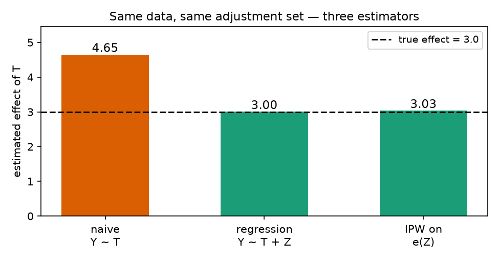
Lecture simulation: \(Y = 3T + 2Z + \varepsilon\), sicker (\(Z\)) more likely treated.
Given a valid \(S\) (ignorability), any of these recovers the effect:
- Regression — include \(S\) as covariates, read the coefficient on \(T\).
- Stratification — effect within strata of \(S\), averaged with population weights (the kidney-stone table).
- Matching on \(S\).
- Propensity score \(e(S) = P(T{=}1 \mid S)\) — match or weight (IPW: \(1/e\) treated, \(1/(1-e)\) control) to build a pseudo-population where \(T \perp S\).
Same \(S\), same answer. A wrong \(S\) gives a wrong answer with a tight standard error — the estimator cannot rescue a bad graph.
Unmeasured confounders: nature’s randomization
Adjustment only blocks paths through variables you measured. Otherwise look for treatment variation that is as good as random:
- Difference-in-differences — change in treated vs. change in control; differences out fixed group differences (Card & Krueger, NJ minimum wage). Assumes parallel trends.
- Instrumental variables — \(Z \to T \to Y\), \(Z \not\to Y\) directly (draft lottery, distance to college). Assumes exclusion.
- Regression discontinuity — treatment switches at a cutoff; compare just above vs. just below. Assumes nothing else jumps there.
Every estimate still rests on assumptions data cannot verify — ignorability, positivity (\(0 < e(S) < 1\)), SUTVA, the graph itself — so state them and stress-test them (sensitivity analysis). Workflow: draw the graph → identify → estimate → refute.
Next session: we leave causal questions for prediction — neural networks: forward pass, loss, gradient descent, by hand.
In-Class Activity
Activity: backdoor identification by hand, then watch a wrong adjustment set lie
Goal: on five DAGs (drawn with networkx), list every backdoor path, mark it open or blocked, code the two rules into a checker, and propose one valid and one invalid adjustment set per DAG. Then simulate data from one of those DAGs with a known effect and estimate it four ways — naive, correct set, wrong set (mediator / collider), inverse-propensity weighting — and see which ones recover the truth.
- Work in groups of 2–3. Open your section’s notebook — the DAG subset and the simulated effect differ by section.
- Parts marked (autograded) are submitted to Gradescope; the rest is participation.
- Staff will circulate — be ready to explain any part of your work.
- Dependencies:
numpy,pandas,matplotlib,networkx,statsmodels,scikit-learn.
Section A1 

Section B1
The activity notebook goes live on the day of the lecture. Colab is optional — you can also open it on GitHub and run it locally.
Going deeper
Full lecture notes: Causal Inference II: Causal Graphs and Estimating Effects
- Reading a causal graph — node, arrow, directed path, descendant, DAG
- Open and blocked paths — the two rules
- The golden rule and Confounders: the backdoor — criterion + adjustment formula
- The backdoor procedure, by hand and the Worked example
- Colliders: adjusting can create bias — the talent/looks simulation
- Regression vs. stratification and Propensity scores — the code the stretch section builds on
- Natural experiments: DiD, IV & RD, and Assumptions you can’t skip
- Where confounding first appeared: Causal Inference I