Recap: Network Centrality and Clustering
DS701 Session 24 — Mon Nov 30, 2026


Today’s plan
- 5 min — knowledge-check review
- 20 min — highlights and Q&A (answer or pass — answering always earns credit)
- 50 min — case study: who should coordinate, and where would the chapter split
- wrap-up and cold-call check-ins; one slide on quiz 3
Knowledge-Check Review
KC 1: Three measures, three notions
The lecture defines three centrality measures — closeness, betweenness, and eigenvector centrality. For each one, state in a single phrase what makes a node score high, and name the karate-club member (0, the instructor, or 33, the president) that each measure ranked first.
KC 2: Why the min cut is useless here
The global minimum cut of the karate-club graph has cost 1: it slices off node 11, which has a single edge. Explain why this “best” cut is useless for partitioning the club, and how the isoperimetric ratio \(\alpha = E(U, V\setminus U)/\min(|U|, |V\setminus U|)\) changes the goal so that a cut like Zachary’s two factions wins instead.
KC 3: Spectral clustering — which eigenvectors, and why they are coordinates
Spectral clustering embeds each node as a point in \(\mathbb{R}^d\) using eigenvectors of the Laplacian \(L = D - A\), then runs \(k\)-means on those points. (a) Which eigenvectors are used, and why is the eigenvector for the smallest eigenvalue excluded? (b) Name the two earlier tools from this course this procedure combines, and say in one sentence why the Laplacian eigenvectors are a sensible set of coordinates for the nodes.
Highlights
1. Centrality — “important” according to whom?
Every measure answers “which nodes matter?” — but each encodes a different notion of mattering:
- closeness — reach: I can get to everyone quickly.
- betweenness — brokerage: traffic has to pass through me.
- eigenvector — status: I am connected to the well-connected.
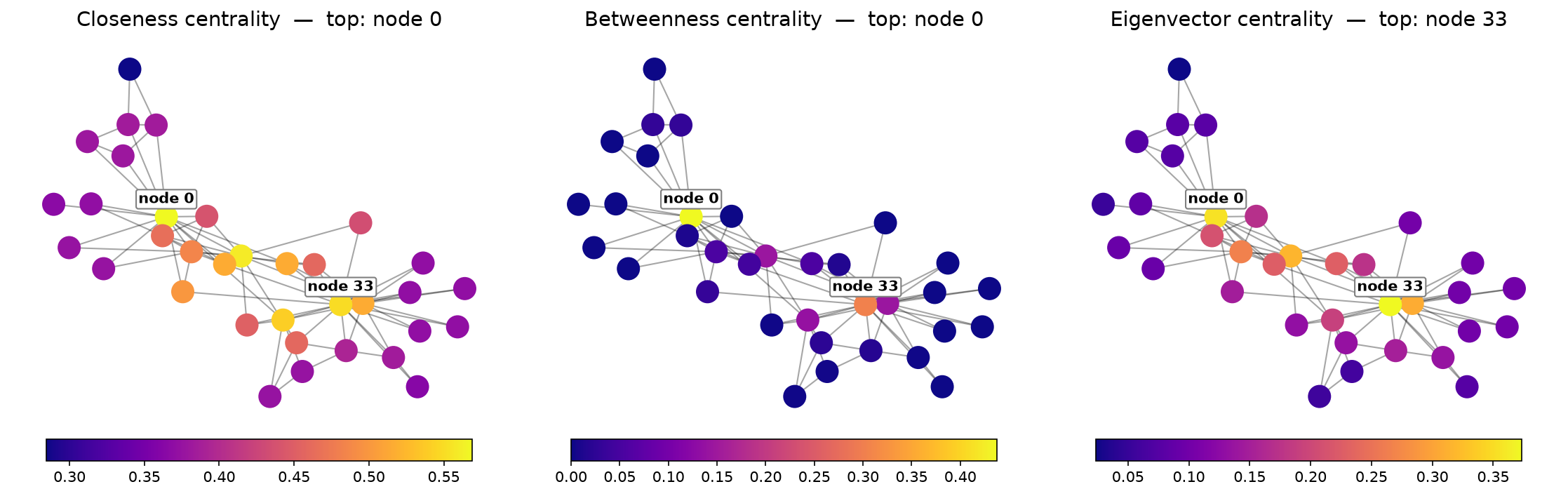
Same club, three colourings. The leaders (0, 33) top everything; the rest of the ranking is where the measures part ways — closeness is nearly flat, betweenness is zero for most and large for two or three brokers, eigenvector centrality lives inside the two dense factions.
2. Eigenvector centrality: importance is recursive
\[ x_i = \frac{1}{\lambda}\sum_{j} A_{ij}\,x_j \qquad\Longleftrightarrow\qquad A\mathbf{x} = \lambda\mathbf{x} \]
- “My score is proportional to the sum of my neighbours’ scores” — a fixed-point condition, and the fixed point is an eigenvector of the adjacency matrix.
- Take the eigenvector of the largest eigenvalue: for a connected graph, Perron–Frobenius guarantees it is the unique eigenvector with all-positive entries — so it reads as a set of importance scores.
- You do not need an eigensolver. Power iteration: start with \(\mathbf{x} = \mathbf{1}/\sqrt{n}\), repeat \(\mathbf{x} \leftarrow A\mathbf{x} / \lVert A\mathbf{x}\rVert\); every step is one round of “pass your score to your neighbours” (the lecture’s \(A\mathbf 1, A^2\mathbf 1, A^3\mathbf 1\) table). Today you will watch it converge to
nx.eigenvector_centralityon a real network.
3. From eigenvector centrality to PageRank
The lecture stops at \(A\mathbf{x} = \lambda\mathbf{x}\); the Web needed two fixes. A random surfer on a page follows a random link with probability \(d\), and jumps to a uniformly random page with probability \(1-d\) (damping, \(d = 0.85\)).
\[ \text{PR}(i) \;=\; \frac{1-d}{n} \;+\; d\sum_{j \to i} \frac{\text{PR}(j)}{\deg^{\text{out}}(j)} \qquad\Longleftrightarrow\qquad \mathbf{r} = \mathbf{G}\,\mathbf{r},\quad \mathbf{G} = d\,A^{T}D^{-1} + \frac{1-d}{n}\mathbf{1}\mathbf{1}^T \]
- Each page splits its score among its out-links (the \(1/\deg\)) — a link from a page that links to everyone is worth little; and the jump term makes the chain irreducible, so a unique stationary vector exists.
- That is eigenvector centrality of a modified matrix: \(\mathbf{r}\) is the eigenvector of the Google matrix \(\mathbf{G}\) for eigenvalue \(1\), and the same power iteration finds it.
- Directed edges (links) are the natural home; on an undirected graph like the karate club it still runs, and it need not agree with eigenvector centrality — today you build it from scratch and check both claims.
4. Cuts: from “cheapest” to “balanced”
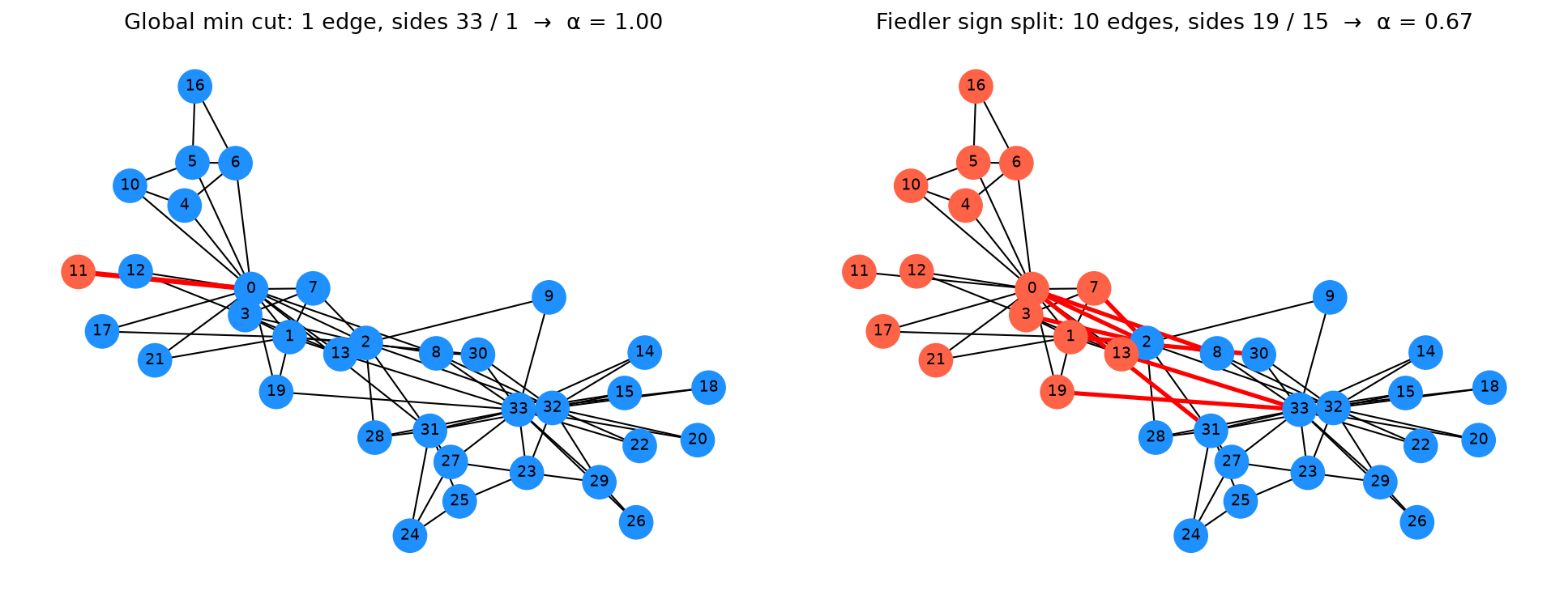
- Min \(s\)–\(t\) cut: fewest edges separating \(s\) from \(t\); polynomial. Zachary’s cut between 0 and 33 predicted the club’s split: all but node 8 with his interaction weights, all but 8 and 9 unweighted.
- Global min cut with no \(s,t\): peels off node 11 for one edge. Cheap, useless.
- Balanced cut: minimise \(\alpha = \dfrac{E(U, V\setminus U)}{\min(|U|, |V\setminus U|)}\) — edges removed per node disconnected. NP-hard → approximate spectrally.
Right panel: the sign of the Fiedler vector on the unweighted karate club, as in the lecture — 10 edges, sides 19 / 15, \(\alpha \approx 0.67\), wrong only about members 2 and 8. No \(s\) or \(t\) was needed.
5. The Laplacian, and why its second eigenvector cuts the graph
\[ L = D - A, \qquad \mathbf{x}^T L\mathbf{x} = \sum_{(i,j)\in E}(x_i - x_j)^2 \;\ge 0 \]
- Symmetric, PSD; \(L\mathbf{1} = \mathbf{0}\), so \(\lambda_1 = 0\) (only once if connected).
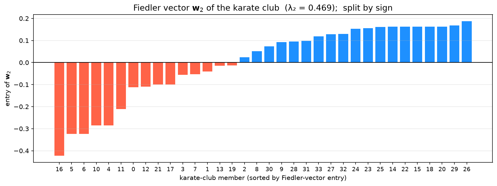
- \(\lambda_2 = \min_{\|\mathbf{x}\|=1,\ \mathbf{x}\perp\mathbf{1}} \mathbf{x}^T L \mathbf{x}\) — the Fiedler value; its eigenvector \(\mathbf{w}_2\) is the smoothest non-constant assignment of numbers to nodes.
- Smooth means neighbours get similar values → the two ends of \(\mathbf{w}_2\) are the two loosely-joined halves. Split by sign (or median, gap, best \(\alpha\)).
6. Spectral clustering is community detection
- \(L = D - A\).
- Eigenvectors of the \(d\) smallest non-zero eigenvalues → columns of \(U \in \mathbb{R}^{n\times d}\).
- Row \(i\) of \(U\) = coordinates of node \(i\).
- \(k\)-means on the \(n\) points.
Football network: sweep \(d\), score against the real conferences with ARI → climbs from 0.32 (\(d = 1\)) to 0.80 (\(d = 3\)), then plateaus near 0.85 from \(d \approx 5\). The gain is in the first few eigenvectors; extra ones neither help nor hurt much. Two-way spectral partitioning is the \(d = 1\), \(k = 2\) special case.
Finding groups of nodes that are densely connected inside and sparsely connected between is called community detection; spectral clustering is one standard method for it, and modularity maximisation (e.g. Louvain, nx.community.louvain_communities) is the other one you will meet most often.
7. The measures disagree — so the question picks the measure
| you are asking … | report |
|---|---|
| who can reach everyone fastest (spread a rumour, place a depot)? | closeness |
| whose removal breaks the most shortest paths (broker, bottleneck, gatekeeper)? | betweenness |
| who is connected to the well-connected (prestige, status)? | eigenvector |
| the same, but each node’s vote is diluted by how many it gives (links, citations)? | PageRank |
| who simply has the most contacts? | degree |
On the karate club the top two agree and hide this. Today’s report-out asks you, from this lecture alone, to describe a network in which they do not — the triangle-with-a-tail already does: node 4 beats nodes 1 and 2 on closeness and betweenness but loses on eigenvector centrality — and then to decide which measure a board asking “who is influential?” should hear about.
In-Class Activity
Activity — Case Study 21: Who Should Coordinate, and Where Would the Chapter Split?
Goal: the community-services nonprofit from Case Study 20 is back — its board wants to name two volunteer coordinators and is weighing a split into two chapters. On the karate club, the public stand-in for its roster: compute closeness, betweenness and eigenvector centrality and see whether they agree on who is central (Part 1); compute the status score by hand with power iteration so the board can be shown where it comes from (Part 2); build PageRank with damping \(d = 0.85\) from scratch and check it against NetworkX (Part 3); partition the network with the Fiedler vector and check the seam against the club’s real split (Part 4) — then write the two sentences at the top of your memo to the board: the two coordinators, by which measure, and the one caveat.
- Work in groups of 2–3. Open your section’s notebook (A1: karate club, B1: Les Misérables).
- Parts marked (autograded) are submitted to Gradescope; the rest is participation.
- Staff will circulate — be ready to explain any part of your work.
- Dependencies:
numpy,pandas,matplotlib,networkx.


The activity notebook goes live on the day of the lecture. Colab is optional — you can also open it on GitHub and run it locally.
Going deeper
Full lecture notes: Network Centrality and Clustering
- Closeness Centrality and Betweenness Centrality — definitions, the dependency ratio, the karate colourings
- Eigenvector Centrality Definition, Matrix Form, Power Iteration and Key Points — \(A\mathbf{x} = \lambda\mathbf{x}\) and Perron–Frobenius
- Centrality Comparison: Karate Example
- Min \(s\)–\(t\) cut, Minimum Cuts and Balanced Cuts — Zachary’s prediction; why min cut peels a leaf
- Spectral Graph Theory, a Laplacian you can check by hand, the Laplacian Quadratic Form and the Fiedler Vector
- Spectral Partitioning — sign / bisection / gap / ratio-cut rules, when they disagree, and the karate split
- Spectral Clustering and its football example with ARI vs. dimension
- Last session’s foundations: Networks I — degree, paths, clustering coefficient, layouts
Before you go: quiz 3 is Wednesday
Wed Dec 2, in class — closed notes, paper and pencil, covering lectures 14–21 (causal inference, neural networks, NLP, recommenders, networks). Today was the last content session.
- The reference sheet for the unit was published last Wednesday: quiz3-reference.pdf. The printed copy handed out on quiz day is identical, and it is the only sheet allowed in the room.
- Today’s ideas that live on the sheet: the three centralities, \(A\mathbf{x} = \lambda\mathbf{x}\), cuts and \(\alpha\), \(L = D - A\), the Fiedler vector, the spectral-clustering steps.
- The homework sets and knowledge checks are the practice; the recap decks are the answer keys.