Network Centrality and Clustering

Overview

We previously introduced the concept of a graph to describe networks. To further analyze networks we will discuss network centrality and clustering.

Motivation

A common question in the analysis of networks is to understand the relative importance of the nodes in the network.

For example:

• in a social network, who are the most influential individuals?
• on the Web, which pages are more informative?
• in road network, which intersections are most heavily used?

The key idea is that the structure of the network should give us some information about the relative importance of the nodes in the network.

Centrality and Clustering

To analyze networks we want to be able to classify:

• important nodes, and
• important groups of nodes.

Determining which nodes are important nodes leads to the notion of centrality.

Determining which groups of nodes are important leads to the notion of clustering and partitioning.

In order to classify important nodes and groups of nodes, we will use graph theory and linear algebra.

Learning Outcomes

By the end of this lecture you should be able to:

• compute closeness, betweenness and eigenvector centrality on a small graph, and say what each one rewards (reach, brokerage, status);
• compute eigenvector centrality by power iteration and check it against NetworkX;
• explain why the minimum cut peels off a leaf, and how the isoperimetric ratio \(\alpha\) rewards balanced cuts;
• build the Laplacian \(L = D - A\), read its Fiedler vector, and split a graph by sign, median or gap;
• run spectral clustering (Laplacian eigenvectors + \(k\)-means) and choose the embedding dimension with the Adjusted Rand Index.

Centrality

Do some nodes in the network have a special role? Are some nodes more important than others?

These are questions of centrality (or prestige).

Definition

• Centrality in graph theory and network analysis refers to measures that identify the most important vertices (nodes) within a graph.
• These measures assign numbers or rankings to nodes based on their position and influence within the network.
• Centrality can help determine which nodes are most influential, critical for connectivity, or central to the flow of information.

We will study three basic notions of centrality:

1. Closeness Centrality: A central node is close to all others.
2. Betweenness Centrality: A central node is on many paths through the network.
3. Eigenvector Centrality: A central node is connected to other central nodes (sometimes called status centrality).

A Graph Small Enough to Do by Hand

A triangle \(1\)–\(2\)–\(3\) with a tail \(3\)–\(4\)–\(5\).

We will compute all three centralities on this graph by hand, then check them with NetworkX.

Notice that nodes 1, 2 and 4 all have degree 2. Watch how the three measures treat them differently.

Karate Club Graph

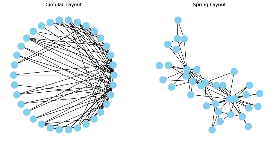
The back story: from 1970 to 1972 the anthropologist Wayne Zachary studied the social relationships inside a university karate club.

While he was studying the club, a factional division led to a splitting of the club in two.

The club became split between those who rallied around the club president and those who rallied around the karate instructor.

You can read the story of the Karate club here. This dataset has become so famous that it has spawned its own academic traditions.

---

Here’s a view of the social network of the karate club.

Gk = nx.karate_club_graph()
fig, (ax1, ax2) = plt.subplots(1, 2, figsize=(12, 6))
nx.draw_networkx(Gk, ax=ax1, pos=nx.circular_layout(Gk),
                 with_labels=False, node_color=OKABE_ITO[1])
ax1.set_title('Circular Layout')
ax1.axis('off')
nx.draw_networkx(Gk, ax=ax2, pos=nx.spring_layout(Gk, seed=9),
                 with_labels=False, node_color=OKABE_ITO[1])
ax2.set_title('Spring Layout')
ax2.axis('off')
plt.show()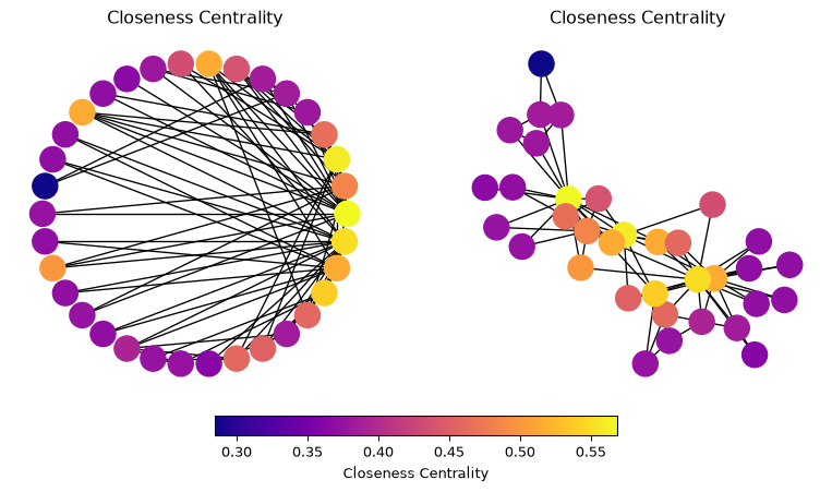

Closeness Centrality

The closeness centrality of a node \(i\) is an indicator of the proximity between node \(i\) and all the other nodes in the graph.

Let \(G=(V, E)\) be a connected graph with \(n\) nodes.

Let \(d(i,j)\) be the shortest path distance between node \(i\) and node \(j\) in \(G\).

The standard way of formulating closeness centrality is the reciprocal of the total distance to all other nodes

\[ \text{closeness}(i) = \frac{1}{\sum_{j \in V} d(i,j)}. \]

By hand. Node 3 is at distances \(1, 1, 1, 2\) from the others: closeness \(1/5\). Node 5 is at \(3, 3, 2, 1\): closeness \(1/9\). All five: \(\left(\tfrac17, \tfrac17, \tfrac15, \tfrac16, \tfrac19\right)\).

NetworkX (and most software) reports the normalised form \((n-1)/\sum_j d(i,j) = 1/\overline{d}(i)\), the reciprocal of the mean distance, so values lie in \((0, 1]\). For node 3 that is \(4/5 = 0.8\).

Interpretation

• Large Closeness Centrality:
  • Indicates that a node is, on average, close to all other nodes in the network.
  • This means it can quickly interact with or reach other nodes.
  • Nodes with high closeness centrality are often considered central or influential because they can efficiently spread information or resources throughout the network.
• Small Closeness Centrality:
  • Indicates that a node is, on average, farther away from all other nodes in the network.
  • These nodes are less central and may take longer to interact with or reach other nodes.
  • Nodes with low closeness centrality are often on the periphery of the network and are less influential in terms of spreading information or resources.

Closeness on the Karate Club

fig = draw_centrality(Gk, nx.closeness_centrality(Gk), 'Closeness centrality')
plt.show()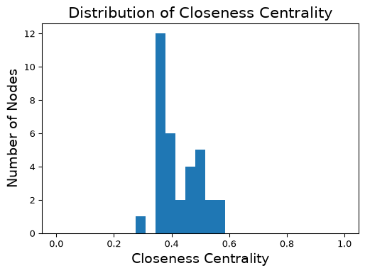

In this graph, most nodes are close to most other nodes: the normalised values only run from about 0.28 to 0.57.

However we can see that some nodes are slightly more central than others.

Betweenness Centrality

Alternatively we might be interested in the question, is the node on many paths?

Betweenness captures how important a node is to the communication process, or how much information passes through the node.

First, let’s consider the case in which there is only one shortest path between any pair of nodes.

Then, the betweenness centrality of node \(i\) is the number of shortest paths that pass through \(i\).

Mathematically, summing over the unordered pairs \(\{j, k\}\) of nodes other than \(i\),

\[ \text{betweenness}(i) = \sum_{\{j,k\} \subseteq V\setminus\{i\}} \begin{cases} 1 &\text{if the path from }j\text{ to }k\text{ goes through }i, \\ 0 &\text{otherwise}. \end{cases} \]

For a graph with \(n\) nodes, we can normalize this to a value between 0 and 1 by dividing by \({n-1 \choose 2} = (n-1)(n-2)/2\), the number of such pairs.

By hand. Node 3 lies on the shortest paths of \(\{1,4\}, \{1,5\}, \{2,4\}, \{2,5\}\): betweenness 4. Node 4 lies on \(\{1,5\}, \{2,5\}, \{3,5\}\): betweenness 3. Nodes 1, 2, 5 lie on none. Normalised by \(\binom42 = 6\): \((0, 0, 0.67, 0.5, 0)\).

General Case: Dependency

In a general graph, there may be multiple shortest paths between \(j\) and \(k\).

To handle this, we define:

• \(\sigma(i \mid j,k)\) is the number of shortest paths between \(j\) and \(k\) that pass through \(i\), and
• \(\sigma(j,k)\) is the total number of shortest paths between \(j\) and \(k\).

Then we define the dependency of \(i\) on the paths between \(j\) and \(k\) as the ratio of those two quantities:

\[ \text{dependency}(i \mid j,k) = \frac{\sigma(i \mid j,k )}{\sigma(j,k)}. \]

You can think of this as the probability that a shortest path between \(j\) and \(k\) goes through \(i\).

General Case: Betweenness Centrality

Finally, the betweenness centrality of node \(i\) is the sum of the dependencies of \(i\) on all pairs of nodes \(j\) and \(k\).

\[ \boxed{\text{betweenness}(i) = \sum_{\{j,k\} \subseteq V\setminus\{i\}} \text{dependency}(i \mid j, k).} \]

Note that many nodes will have a betweenness centrality of zero – no shortest paths go through them.

Betweenness on the Karate Club

fig = draw_centrality(Gk, nx.betweenness_centrality(Gk), 'Betweenness centrality')
plt.show()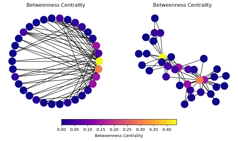

We start to see with this metric the importance of two or three key members of the karate club; most members are on almost no shortest paths.

Eigenvector Centrality

Eigenvector centrality is a measure used in network analysis to determine the influence of a node within a network.

The centrality score of a node is proportional to the sum of the centrality scores of its neighbors.

The main idea of eigenvector (or status) centrality is that high status nodes are connected to high status nodes.

We calculate this with some matrix algebra.

Reminder: The Adjacency Matrix

An \(n\)-node undirected graph \(G = (V, E)\) has adjacency matrix

\[ A_{ij} = \begin{cases} 1, & \text{if $(i, j)\in E$ }\\ 0, & \text{otherwise} \end{cases}. \]

• Row sums are degrees, and column \(j\) holds \(j\)’s neighbors.
• For an undirected graph \(A\) is nonnegative and symmetric.

See the adjacency matrix in Networks I for the worked five-node example.

Reminder: Properties of nonnegative symmetric matrices

A nonnegative symmetric matrix \(A\) has the following properties:

1. All eigenvalues of \(A\) are real, and its eigenvectors can be chosen orthogonal (symmetric matrices, Lecture 12).
2. The largest eigenvalue of \(A\) is nonnegative, and no other eigenvalue exceeds it in absolute value. (The other eigenvalues can be negative: a single edge has eigenvalues \(1\) and \(-1\).)
3. If the graph is connected, the largest eigenvalue has an eigenvector with all positive entries, and it is the only eigenvector with all positive entries.

This is a consequence of the Perron-Frobenius Theorem.

Eigenvector Centrality Definition

Given a graph with \(n\) nodes and let \(A\) be the adjacency matrix of the graph.

The eigenvector centrality \(x_i\) of node \(i\) is defined as proportional to the sum of the centrality scores of its neighbors.

\[ x_i = \frac{1}{\lambda} \sum_{j=1}^{n} A_{ij} x_j, \]

where

• \(x_i\) is called the eigenvector centrality of node \(i\).
• \(\lambda\) is a constant (which we’ll show is an eigenvalue).

Put another way, the importance of node \(i\) is proportional to the sum of the importance of the other nodes \(j\) directly connected to \(i\).

Matrix Form

In matrix form, this can be written as

\[ \mathbf{Ax} = \lambda \mathbf{x}, \]

where \(\mathbf{x}\) is the eigenvector corresponding to the eigenvalue \(\lambda\) of the adjacency matrix \(\mathbf{A}\).

The eigenvector \(\mathbf{x}\) gives the centrality scores for all nodes in the network.

• In general, there may be multiple eigenvalues \(\lambda\) for which the above equation holds.
• We use the largest eigenvalue: by Perron–Frobenius its eigenvector is the only one whose entries are all positive, so it is the only one that reads as a set of scores.

Computing It: Power Iteration

Start from \(\mathbf{x} = \mathbf{1}\) and repeat \(\mathbf{x} \leftarrow A\mathbf{x}\), rescaling each time. One multiplication = every node replaces its score by the sum of its neighbours’ scores.

	node 1	node 2	node 3	node 4	node 5
\(A\mathbf 1\) (= degrees)	2	2	3	2	1
\(A^2\mathbf 1\)	5	5	6	4	2
\(A^3\mathbf 1\)	11	11	14	8	4
\(A^3\mathbf 1\), rescaled so max = 1	0.79	0.79	1	0.57	0.29
converged (NetworkX), max = 1	0.82	0.82	1	0.57	0.26

Nodes 1, 2 and 4 all start at degree 2, but node 4 falls behind: its neighbours are node 3 and the leaf 5, while 1 and 2 are attached to each other and to node 3.

Why it works. Write \(\mathbf 1 = \sum_k c_k \mathbf{v}_k\) in eigenvectors; then \(A^t\mathbf 1 = \sum_k c_k\lambda_k^t\mathbf{v}_k\), and the largest eigenvalue (here \(\lambda = 2.21\)) dominates as \(t\) grows. Perron–Frobenius makes \(c_1 > 0\), since \(\mathbf v_1\) is positive.

Three Measures, One Graph

A = nx.to_numpy_array(T, nodelist=[1, 2, 3, 4, 5])
x = np.ones(5)
for _ in range(100):                     # power iteration
    x = A @ x
    x = x / np.linalg.norm(x)

ec = nx.eigenvector_centrality(T)
table = pd.DataFrame({
    'degree': dict(T.degree()),
    'closeness 1/Σd': {v: 1 / sum(d.values()) for v, d in nx.shortest_path_length(T)},
    'betweenness (raw)': nx.betweenness_centrality(T, normalized=False),
    'eigvec, power iter.': dict(zip(T, x / x.max())),
    'eigvec, NetworkX': {v: ec[v] / max(ec.values()) for v in T},
})
print(table.round(3))

   degree  closeness 1/Σd  betweenness (raw)  eigvec, power iter.  \
1       2           0.143                0.0                0.824   
2       2           0.143                0.0                0.824   
3       3           0.200                4.0                1.000   
4       2           0.167                3.0                0.567   
5       1           0.111                0.0                0.256   

   eigvec, NetworkX  
1             0.824  
2             0.824  
3             1.000  
4             0.567  
5             0.256  

Node 3 wins everything. Node 4 beats nodes 1 and 2 on closeness and betweenness (it sits on the way to node 5) but loses on eigenvector centrality (its neighbours are poorer). Each measure encodes a different notion of importance.

Key Points on Eigenvector Centrality

• Eigenvector: The vector \(\mathbf{x}\) represents the centrality scores.
• Largest Eigenvalue: The centrality scores are derived from the eigenvector corresponding to the largest eigenvalue of the adjacency matrix.
• Perron-Frobenius Theorem: For a connected graph, the largest eigenvalue is positive. In addition, there is only 1 corresponding eigenvector with all positive entries.
• Power iteration finds it with nothing but matrix–vector products, which is how it is computed on large graphs.

The Perron-Frobenius Theorem is an important theoretical tool when working with adjacency matrices, which are by definition nonnegative.

Eigenvector Centrality: Example

fig = draw_centrality(Gk, nx.eigenvector_centrality(Gk), 'Eigenvector centrality')
plt.show()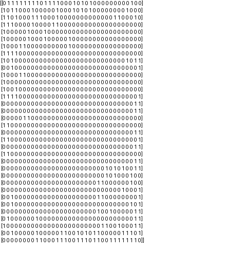

Centrality Comparison: Karate Example

Let’s compare the three versions of centrality we’ve looked at so far.

fn = [nx.closeness_centrality, nx.betweenness_centrality, nx.eigenvector_centrality]
title = ['Closeness Centrality', 'Betweenness Centrality', 'Eigenvector Centrality']
pos = nx.spring_layout(Gk, seed=9)
#
fig, axs = plt.subplots(2, 3, figsize = (14, 8))
for i in range(3):
    cent = list(fn[i](Gk).values())
    nx.draw_networkx(Gk, ax = axs[0, i],
                 pos = pos,
                 node_color = cent,
                 cmap = plt.cm.plasma,
                 with_labels = False)
    axs[0, i].set_title(title[i], size = 14)
    axs[0, i].axis('off')
    #
    axs[1, i].hist(cent, bins=np.linspace(0, 1, 30), color=OKABE_ITO[5])
    axs[1, i].set_ylim([0, 27])
    axs[1, i].set_xlabel(title[i], size = 14)
axs[1, 0].set_ylabel('Number of Nodes', size = 14)
plt.show()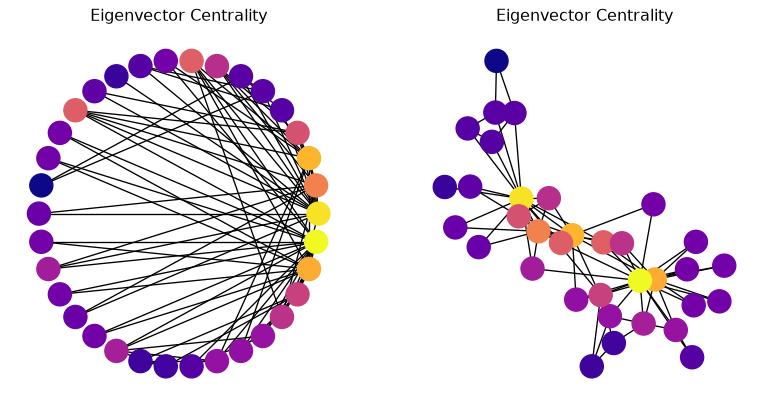

It appears that we have identified the instructor (node 0) and the club president (node 33) as important nodes based on all three measures. The rest of the ranking is where the measures part ways.

Clustering and Partitioning

Clustering and Partitioning

We now turn to the question of finding important groups of nodes.

Why might we want to cluster graph nodes?

• Assigning computations to processors in a parallel computer
• Segmenting images (finding boundaries between objects)
• Clustering words found together in documents, or documents with similar words
• Divide and conquer algorithms
• Circuit layout in VLSI
• Community detection in social networks

Min \(s\)-\(t\) cut

We’ll start with a problem that is fundamental to many other problems in graph analysis.

It involves finding the smallest set of edges that, if removed, would disconnect a specified source node (s) from a target node (t) in a graph.

The goal of a min \(s\)-\(t\) cut is to partition the graph into two disjoint subsets such that:

• \(s\) is in one subset and \(t\) is in the other, and
• the total weight (or number) of the edges that need to be removed to achieve this separation is minimized.

Practical Example: Soviet Railway Network

Here is a schematic diagram of the railway network of the Western Soviet Union and Eastern European countries in the Cold War era.

The idea was to determine a minimum cut, which would best halt the flow of materials in the railway network.

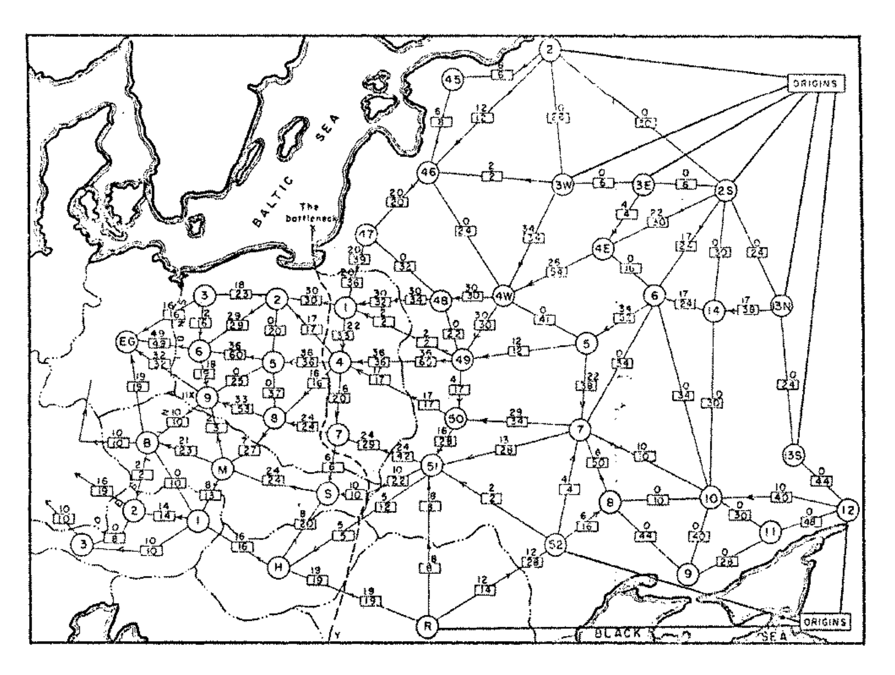
For an interesting historical perspective on the min-cut problem and its relation to the Cold War, see “On the history of the transportation and maximum flow problems,” by Alexander Schrijver, in Mathematical Programming 91.3 (2002): 437-445.

Cost of a Cut

Let \(G = (V, E)\) be a weighted graph.

A weighted graph assigns a weight \(w(e)\) to each edge \(e\in E\).

An \(s\)-\(t\) cut \(C\) of \(G\) is a partition of \(V\) into \((U, V-U)\) such that \(s \in U\) and \(t \in V-U\).

The cost of a cut is the total weight of the edges that go between the two parts:

\[ \text{Cost}(C) = \sum_{e(u,v),\, u\in U,\, v\in V-U} w(e). \]

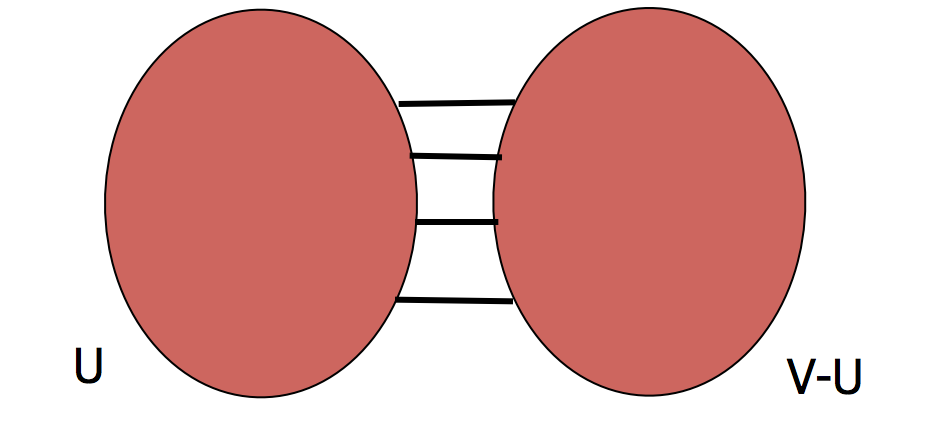
For unweighted graphs, we can set \(w(e) = 1\) for all edges, so the cost becomes the number of edges that cross the cut.

Min \(s\)-\(t\) Cut Problem

Let \(G = (V, E)\) be a weighted graph with edge weights \(w(e)\) for each \(e \in E\).

An \(s\)-\(t\) cut \(C\) is a partition of \(V\) into \((U, V-U)\) such that \(s \in U\) and \(t \in V-U\).

The min \(s\)-\(t\) cut problem seeks to find the partition that minimizes this cost:

\[ \boxed{\min_{C} \text{Cost}(C) = \min_{U \subseteq V: s \in U, t \notin U} \sum_{e(u,v),\, u\in U,\, v\in V-U} w(e).} \]

This is a very famous problem that can be solved in time that is polynomial in the number of nodes \(|V|\) and edges \(|E|\).

Increasingly better solutions have been found over the past 60+ years.

---

What can a min \(s\)-\(t\) cut tell us about a graph?

Let’s look at the karate club, in which we’ve highlighted the instructor (node 0, orange-red) and the president (node 33, blue).

G = nx.karate_club_graph()
pos = nx.spring_layout(G, seed=9)
side_colors = [OKABE_ITO[3], OKABE_ITO[5]]   # instructor's side, president's side
#
node_color = 34 * ['lightgray']
node_color[0], node_color[33] = side_colors
fig = plt.figure(figsize=(10, 5))
nx.draw_networkx(G, pos=pos,
                 with_labels=True, node_size=1000,
                 node_color = node_color,
                 font_size=16)
plt.axis('off')
plt.show()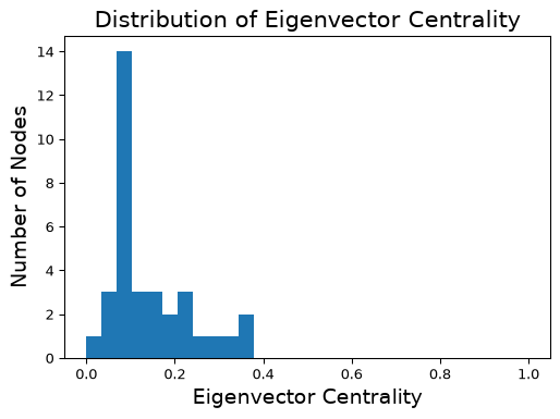

---

As mentioned, when Wayne Zachary studied the club, a conflict arose between the instructor and the president (nodes 0 and 33, respectively).

Zachary predicted the way the club would split based on an \(s\)-\(t\) min cut between the instructor and the president.

cut_edges = nx.minimum_edge_cut(G, s=0, t=33)
Gcopy = G.copy()
Gcopy.remove_edges_from(cut_edges)
instructor_side = nx.node_connected_component(Gcopy, 0)
node_colors = [side_colors[0] if v in instructor_side else side_colors[1] for v in G]
fig = plt.figure(figsize=(12, 5))
nx.draw_networkx(G, node_color=node_colors, pos=pos,
                 with_labels=True, node_size=1000, font_size=16)
plt.axis('off')
plt.show()
wrong = [v for v in G if (v in instructor_side) != (G.nodes[v]['club'] == 'Mr. Hi')]
print(f'{len(cut_edges)} cut edges; members on the wrong side of the actual split: {wrong}')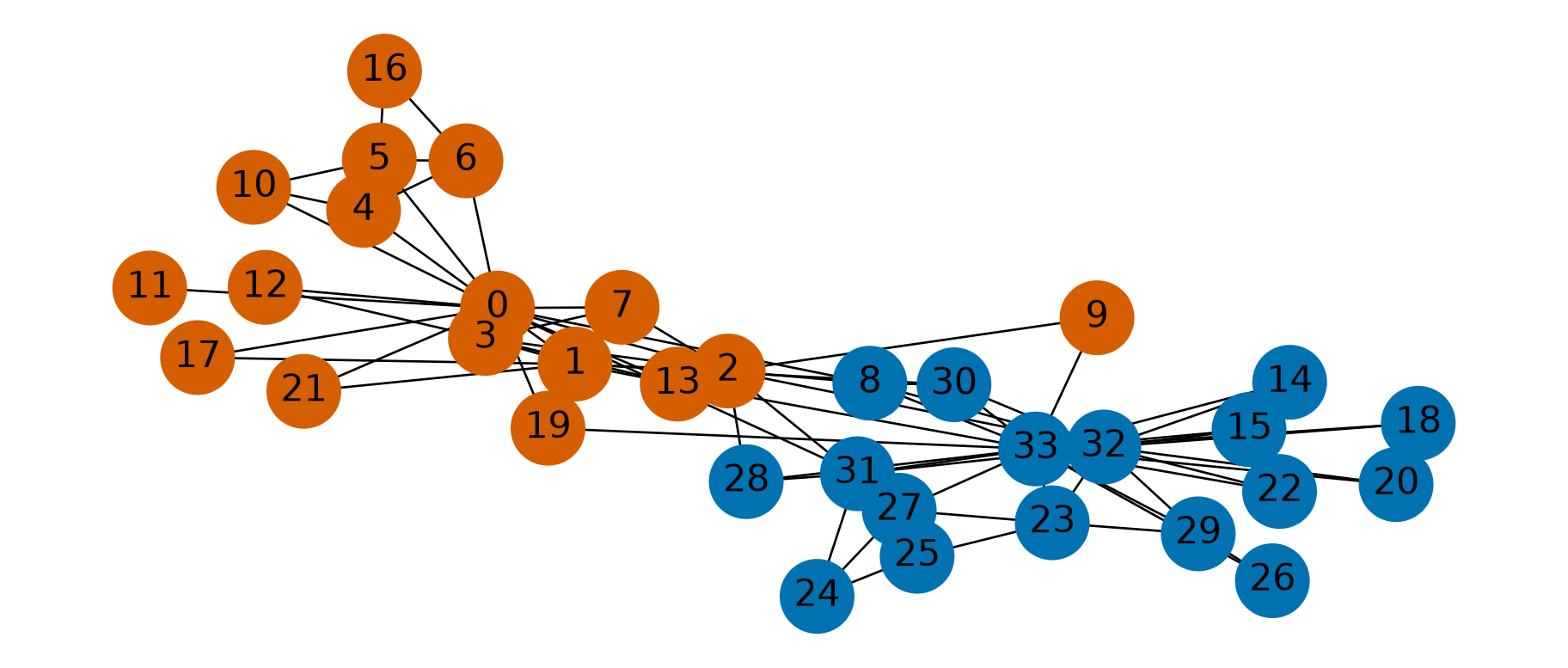

10 cut edges; members on the wrong side of the actual split: [8, 9]

This unweighted cut places every member correctly except two (8 and 9). Zachary’s edges carried interaction counts, which he used as capacities; with those weights the min cut misses only node 8.

Minimum Cuts

In partitioning a graph, we may not have any particular \(s\) and \(t\) in mind.

Rather, we may want to simply find the minimal way to disconnect the graph.

Clearly, we can do this using an \(s\)-\(t\) min cut, by simply trying all \(s\) and \(t\) pairs.

---

Let’s try this approach of finding the minimum \(s-t\) cut over all possibilities in the karate club graph.

Gcopy = G.copy()
Gcopy.remove_edges_from(nx.minimum_edge_cut(G))
big_side = max(nx.connected_components(Gcopy), key=len)
node_colors = [side_colors[1] if v in big_side else side_colors[0] for v in G]
fig = plt.figure(figsize=(12,5))
nx.draw_networkx(G, node_color=node_colors, pos=pos, with_labels=True,
                 node_size=1000, font_size=16)
plt.axis('off')
plt.show()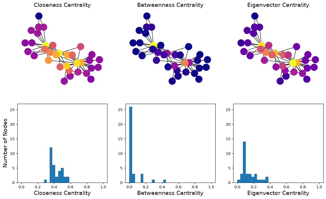

This is in fact the minimum cut. Node 11 only has one edge to the rest of the graph, so the min cut is 1.

---

As this example shows, minimum cut is not, in general, a good approach for clustering or partitioning.

To get a more useful partition, we need to define a new goal. The new goal will be to find a balanced cut.

Balanced Cuts

The idea to avoid the problem above is to normalize the cut by the size of the smaller of the two components. The problem above would be avoided because the smaller of the two cuts is just a single node.

This leads us to define the isoperimetric ratio

\[ \alpha = \frac{E(U, V\setminus U)}{\min(|U|, |V\setminus U|)}, \]

and the isoperimetric number of G

\[ \alpha(G) = \min_U \frac{E(U, V\setminus U)}{\min(|U|, |V\setminus U|)}, \]

where \(E(U, V\setminus U)\) is the number of edges between the two parts.

The idea is that finding \(\alpha(G)\) gives a balanced cut – one that maximizes the number of disconnected nodes per edge removed.

---

Unfortunately, this is a challenging problem that is not computable in polynomial time.

However, we can make good approximations, which we’ll look at now.

To do so, we’ll introduce spectral graph theory.

Spectral Graph Theory

Spectral graph theory is the use of linear algebra to study the properties of graphs.

To introduce spectral graph theory, we define some terms.

Let \(G\) be an undirected graph with \(n\) nodes. We define the \(n\times n\) matrix \(D\) as a diagonal matrix of node degrees, i.e., \(D = \text{diag}(d_1, d_2, d_3, \dots)\) where \(d_i\) is the degree of node \(i\).

Assuming \(G\) has adjacency matrix \(A\), we define the Laplacian of \(G\) as

\[ L = D - A. \]

So \(L_{ii} = d_i\) on the diagonal; off the diagonal, \(L_{ij} = -1\) if \((i,j)\) is an edge and \(0\) otherwise. Every row sums to zero.

If you want to study this in more detail, some excellent references are

• Allow Me to Introduce Spectral and Isoperimetric Graph Partitioning by Jonathan Shewchuck, which has outstanding visualizations and physical intuition.
• Spectral and Algebraic Graph Theory by Daniel Spielman which provides proofs and much more detail.

A Laplacian You Can Check by Hand

The graph from Homework 10, Problem 3: two triangles joined by the bridge \(3\)–\(4\). Degrees \((2,2,3,3,2,2)\).

\[ L = D - A = \begin{bmatrix} \phantom{-}2&-1&-1&\phantom{-}0&\phantom{-}0&\phantom{-}0\\ -1&\phantom{-}2&-1&\phantom{-}0&\phantom{-}0&\phantom{-}0\\ -1&-1&\phantom{-}3&-1&\phantom{-}0&\phantom{-}0\\ \phantom{-}0&\phantom{-}0&-1&\phantom{-}3&-1&-1\\ \phantom{-}0&\phantom{-}0&\phantom{-}0&-1&\phantom{-}2&-1\\ \phantom{-}0&\phantom{-}0&\phantom{-}0&-1&-1&\phantom{-}2 \end{bmatrix} \]

Each row: the degree on the diagonal, a \(-1\) for each neighbour, and a row sum of zero.

Laplacian Matrix Interpretation

Now let us think about an \(n\)-component vector \(\mathbf{x} \in \mathbb{R}^n\) as an assignment of values to nodes in the graph \(G\).

For example, \(\mathbf{x}\) could encode node importance or strength or even a more concrete notion like temperature or altitude.

Laplacian Quadratic Form

Here is an amazing fact about the Laplacian of \(G\).

The quadratic form

\[ \mathbf{x}^TL\mathbf{x} = \sum_{(i,j)\in E} (x_i - x_j)^2, \]

i.e., \(\mathbf{x}^TL\mathbf{x}\) is the sum of squared differences of \(\mathbf{x}\) over the edges in \(G\).

On the two-triangle graph, take \(\mathbf{x} = (1, 1, 1, -1, -1, -1)\). Every edge inside a triangle contributes \(0\); only the bridge contributes, \((1-(-1))^2 = 4\). So \(\mathbf{x}^TL\mathbf{x} = 4\).

Proof that Quadratic Form is Sum of Squared Differences

To see that

\[ \mathbf{x}^TL\mathbf{x} = \sum_{(i,j)\in E} (x_i - x_j)^2, \]

first consider \(\mathbf{x}^TL\mathbf{x}\). Writing out the quadratic form explicitly, we have that

\[ \mathbf{x}^TL\mathbf{x} = \sum_{i, j} L_{ij}x_i x_j. \]

Now, taking into account the values in \(L\), we see that in the sum we will have the term \(d_i x_i^2\) for each \(i\), and also 2 terms of \(-x_ix_j\) whenever \((i,j)\in E\).

Turning to

\[\sum_{(i,j)\in E} (x_i - x_j)^2 = \sum_{(i,j)\in E} x_i^2 - 2x_ix_j + x_j^2, \]

we have the same set of terms in the sum.

---

Now, let’s think about a vector \(\mathbf{x}\) that minimizes the differences over the edges in the graph.

Remember that the \(x_i\) are the values at nodes \(i\) in the graph, which we can think of as a function on the graph.

We want these functions to be smooth – neighboring nodes don’t differ too much in their \(x\) values.

To enforce this smoothness we want to minimize the sum of the squared differences between neighboring nodes.

\[ \min_{\Vert \mathbf{x}\Vert = 1}\sum_{(i,j)\in E} (x_i - x_j)^2. \]

We constrain \(\mathbf{x}\) to have a nonzero norm (i.e. \(\Vert \mathbf{x}\Vert = 1\)), otherwise \(\mathbf{x} = \mathbf{0}\) would be a trivial solution.

---

We can express this in terms of the graph Laplacian:

\[ \min_{\Vert \mathbf{x}\Vert = 1}\sum_{(i,j)\in E} (x_i - x_j)^2 = \min_{\Vert \mathbf{x}\Vert = 1} \mathbf{x}^TL\mathbf{x}. \]

For a symmetric matrix, the minimum of \(\mathbf{x}^TL\mathbf{x}\) over unit vectors is

\[ \lambda = \min_{\Vert \mathbf{x}\Vert = 1} \mathbf{x}^TL\mathbf{x}, \]

the smallest eigenvalue of \(L\), attained at the corresponding eigenvector.

This is PCA’s variance argument from Lecture 13 run backwards: there the top eigenvector of the covariance matrix maximised \(\mathbf{w}^TS\mathbf{w}\); here the bottom eigenvector of \(L\) minimises \(\mathbf{x}^TL\mathbf{x}\).

We are connecting functions on the graph \(G\) with eigenvectors of the matrix \(L\). This is quite remarkable.

---

What do we know about \(L\)?

1. \(L\) is symmetric. Therefore the eigenvectors of \(L\) are orthogonal and its eigenvalues are real (Lecture 12).
2. \(L\) is positive semidefinite, i.e. \(\mathbf{x}^T L\mathbf{x} \geq 0\) for all \(\mathbf{x}\).
   • Therefore the eigenvalues of \(L\) are all nonnegative.

We can order the eigenvalues from largest to smallest \(\lambda_n \geq \dots \geq \lambda_2 \geq \lambda_1 \geq 0.\)

How do we know that \(L\) is positive semidefinite?

• Consider \(\sum_{(i,j)\in E} (x_i - x_j)^2.\) This is always a nonnegative quantity.
• As a result, \(\mathbf{x}^T L\mathbf{x} \geq 0\) for all \(\mathbf{x}\).

---

Assume that \(G\) is connected (i.e. there is a path between any two nodes).

Then \(L\) has a single eigenvalue of value \(\lambda_1 = 0\). The corresponding eigenvector is \(\mathbf{w}_1 = \mathbf{1} = [1, 1, 1, \dots]^T\).

It is easy to verify that

\[ L{\mathbf 1}=0 \cdot {\mathbf 1} = {\mathbf 0}. \]

Recall that row \(i\) of \(L\) consists of \(d_i\) on the diagonal, and \(d_i\) -1s in other positions.

---

The second-smallest eigenvalue of \(L\), \(\lambda_2\), is called the Fiedler value.

We know that all of the other eigenvectors of \(L\) are orthogonal to \(\mathbf 1\), because \(L\) is symmetric.

As a result, a definition of the second smallest eigenvalue is:

\[ \lambda_2 = \min_{\Vert \mathbf{x}\Vert = 1, \;\mathbf{x}\perp {\mathbf 1}} \mathbf{x}^TL\mathbf{x}. \]

Note that \(\mathbf{x} \perp {\mathbf 1}\) means that the sum of the entries in \(\mathbf{x}\) is zero, which implies that \(\mathbf{x}\) is mean-centered.

Fiedler Vector

The corresponding eigenvector to \(\lambda_2\) is called the Fiedler vector.

It minimizes

\[ \mathbf{w}_2 = \arg \min_{\Vert \mathbf{x}\Vert=1,\;\mathbf{x}\perp {\mathbf 1}} \sum_{(i,j)\in E} (x_i - x_j)^2. \]

If we think of \(x_i\) as a 1-D coordinate for node \(i\) in the graph, then choosing \(\mathbf{x} = \mathbf{w}_2\) (the eigenvector corresponding to \(\lambda_2\)) puts each node in a position that minimizes the sum of the squared stretching of each edge.

The Fiedler Vector of the Two-Triangle Graph

L = nx.laplacian_matrix(H, nodelist=[1, 2, 3, 4, 5, 6]).toarray()
lam, W = np.linalg.eigh(L)          # eigenvalues in increasing order
w2 = W[:, 1] * np.sign(W[0, 1])     # an eigenvector's sign is arbitrary: make node 1 positive
print('eigenvalues:', np.clip(lam, 0, None).round(3))   # clip round-off below 0
print('w2:         ', w2.round(3))

eigenvalues: [0.    0.438 3.    3.    3.    4.562]
w2:          [ 0.465  0.465  0.261 -0.261 -0.465 -0.465]

• \(\lambda_1 = 0\) (connected graph) and the Fiedler value is \(\lambda_2 = 0.438\), small because one edge holds the graph together.
• \(\mathbf{w}_2 = (0.465, 0.465, 0.261, -0.261, -0.465, -0.465)\): one triangle positive, the other negative; the bridge endpoints 3 and 4 sit closest to zero.
• The entries sum to zero (\(\mathbf{w}_2 \perp \mathbf 1\)). Flipping every sign gives the same eigenvector.

Spectral Layout = \((\mathbf{w}_2, \mathbf{w}_3)\)

Recall from physics that the energy in a stretched spring is proportional to the square of its stretched length. Placing the nodes at \(\mathbf{w}_2\) is a spring-energy layout in one dimension: springs only, with the constraints \(\Vert\mathbf{x}\Vert = 1\) and \(\mathbf{x}\perp\mathbf 1\) doing the job of repulsion. The spring layout you saw last lecture adds explicit repulsion between nodes, which is why the two pictures differ.

The spectral layout from last lecture uses \(\mathbf{w}_2\) for the first coordinate and \(\mathbf{w}_3\) for the second, where \(\lambda_3 = \min_{\Vert \mathbf{x}\Vert = 1, \;\mathbf{x}\perp \{\mathbf{1}, \mathbf{w}_2\}} \mathbf{x}^TL\mathbf{x}\).

import os, urllib.request

def data_file(path):
    """Course data file: use a local copy (here, or in the repo root above a
    notebook in jupyter_notebooks/), else fetch it from the Materials repo (Colab)."""
    for prefix in ('', '../'):
        if os.path.exists(prefix + path):
            return prefix + path
    os.makedirs(os.path.dirname(path) or '.', exist_ok=True)
    urllib.request.urlretrieve(
        'https://raw.githubusercontent.com/tools4ds/DS701-Materials-FA26/main/' + path, path)
    return path

import re
import matplotlib.patches as mpatches
from matplotlib.colors import ListedColormap

# data from http://www-personal.umich.edu/~mejn/netdata/
football = nx.read_gml(data_file('data/football.gml'))
conf = np.array([d['value'] for _, d in football.nodes.data()])
conf_name = {}
with open(data_file('data/football.txt'), 'r') as fp:
    for line in fp:
        m = re.match(r'\s*(\d+)\s+=\s*([\w\s-]+)\s*\n', line)
        if m:
            conf_name[int(m.group(1))] = m.group(2).strip()

colours = list(CATEGORICAL_12)
colours[5], colours[8] = colours[8], colours[5]   # Independents (5) in grey: not a conference
conf_cmap = ListedColormap(colours)
conf_patches = [mpatches.Patch(color=conf_cmap(i), label=conf_name[i]) for i in range(12)]

def draw_football(ax, pos, labels, title, edges=True):
    nx.draw_networkx_nodes(football, pos=pos, ax=ax, node_size=40,
                           node_color=[conf_cmap(int(c)) for c in labels])
    if edges:
        nx.draw_networkx_edges(football, pos=pos, ax=ax, edge_color='gray', alpha=0.3)
    ax.set_title(title, size=14)
    ax.axis('off')

fig, axes = plt.subplots(1, 2, figsize=(13, 6))
draw_football(axes[0], nx.spectral_layout(football), conf, 'Spectral layout $(\\mathbf{w}_2, \\mathbf{w}_3)$')
draw_football(axes[1], nx.spring_layout(football, seed=0), conf, 'Spring layout')
fig.legend(handles=conf_patches, loc='lower center', ncol=6, fontsize=10)
plt.subplots_adjust(bottom=0.15)
plt.show()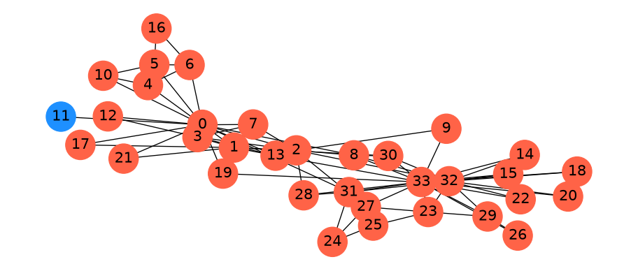

Spectral Partitioning

This leads to key ideas in node partitioning.

The basic idea is to partition nodes according to the Fiedler vector \(\mathbf{w}_2\).

There are a number of options for how to split based on the Fiedler vector.

If \(\mathbf{w}_2\) is the Fiedler vector, then split nodes according to a value \(s\):

• bisection: \(s\) is the median value in \(\mathbf{w}_2\)
• sign: separate positive and negative values (\(s = 0\))
• gap: separate according to the largest gap in the values of \(\mathbf{w}_2\)
• ratio cut (sweep): try every threshold \(s\) and keep the one that minimizes the isoperimetric ratio \(\alpha\). The sweep is the version with a performance guarantee (Cheeger’s inequality).

See Spectral and Algebraic Graph Theory by Daniel Spielman. Chapter 20 proves a lower bound: every \(U\) with \(|U| \leq |V|/2\) has ratio \(\alpha(U) \geq \lambda_2 (1-s)\), where \(s = |U|/|V|\), so \(\alpha(G) \geq \lambda_2/2\). Cheeger’s inequality gives the matching upper bound: the best threshold cut of \(\mathbf{w}_2\) has \(\alpha \le \sqrt{2 d_{\max} \lambda_2}\).

Splitting the Two-Triangle Graph

\[ \mathbf{w}_2 = (\underbrace{0.465,\ 0.465,\ 0.261}_{\text{nodes } 1,2,3},\ \underbrace{-0.261,\ -0.465,\ -0.465}_{\text{nodes } 4,5,6}) \]

• Sign (\(s = 0\)): \(\{1,2,3\} \mid \{4,5,6\}\).
• Bisection (median \(= 0\)): the same split, 3 and 3.
• Gap: the largest gap is \(0.261 - (-0.261) = 0.522\), between nodes 3 and 4: the same split.
• All three cut only the bridge: \(\alpha = 1/\min(3,3) = 1/3\), which is the best possible here.

When the Rules Disagree

# K3 = {1, 2, 3} and K5 = {4, ..., 8}, joined by the bridge 3-4
K = nx.complete_graph([1, 2, 3])
K.add_edges_from(nx.complete_graph([4, 5, 6, 7, 8]).edges())
K.add_edge(3, 4)
nodes = list(range(1, 9))
lam_K, W_K = np.linalg.eigh(nx.laplacian_matrix(K, nodelist=nodes).toarray())
f = W_K[:, 1] * -np.sign(W_K[0, 1])           # make node 1 negative

def alpha(G, U):
    cut = sum((a in U) != (b in U) for a, b in G.edges())
    return cut, cut / min(len(U), G.number_of_nodes() - len(U))

splits = {'sign / gap': {v for v, fv in zip(nodes, f) if fv < 0},
          'bisection (median)': {v for v, fv in zip(nodes, f) if fv < np.median(f)}}
pos_K = nx.spring_layout(K, seed=2)
fig, axes = plt.subplots(1, 2, figsize=(12, 4.5))
for ax, (name, U) in zip(axes, splits.items()):
    cut, a = alpha(K, U)
    nx.draw_networkx(K, pos=pos_K, ax=ax, node_size=700, font_size=14,
                     node_color=[OKABE_ITO[3] if v in U else OKABE_ITO[5] for v in K])
    ax.set_title(f'{name}: {cut} cut edge(s), α = {a:.2f}', size=14)
    ax.axis('off')
plt.show()
print('w2 =', f.round(2))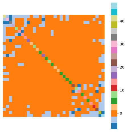

w2 = [-0.51 -0.51 -0.32  0.18  0.29  0.29  0.29  0.29]

\(K_3\) and \(K_5\) joined by one edge. The bridge is still the natural cut, and sign and gap find it (\(\alpha = 1/3\)). Bisection insists on 4 and 4, so it must cut four edges inside the \(K_5\) (\(\alpha = 1\)). Balance costs edges.

---

Here is a spectral partitioning for the karate club graph, splitting by sign.

f = nx.fiedler_vector(G, weight=None, seed=0)   # unweighted, like L = D - A above
if f[0] > 0:
    f = -f                                    # put the instructor on the negative side
U = {v for v in G if f[v] < 0}
#
fig = plt.figure(figsize=(12,5))
node_colors = [side_colors[0] if v in U else side_colors[1] for v in G]
nx.draw_networkx(G, pos=pos, node_color=node_colors, with_labels=True,
        node_size=1000, font_size=16)
plt.axis('off')
plt.show()
cut, a = alpha(G, U)
wrong = [v for v in G if (v in U) != (G.nodes[v]['club'] == 'Mr. Hi')]
print(f'sides {len(U)} / {34 - len(U)}, {cut} cut edges, alpha = {a:.2f}; '
      f'on the wrong side of the actual split: {wrong}')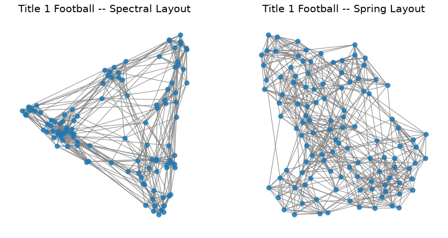

sides 15 / 19, 10 cut edges, alpha = 0.67; on the wrong side of the actual split: [2, 8]

With no \(s\) or \(t\) specified, the sign of \(\mathbf{w}_2\) recovers the club’s actual split except for two members, nearly the same partition as the \(s\)-\(t\) min cut between the instructor and the president.

NetworkX ships the karate club with edge weights (interaction counts), and nx.laplacian_matrix and nx.fiedler_vector use them by default. We pass weight=None so that the computation matches \(L = D - A\) with \(A_{ij} \in \{0, 1\}\).

Spectral Clustering

In many cases we would like to move beyond graph partitioning, to allow for clustering nodes into, say, \(k\) clusters.

The idea of spectral clustering takes the observations about the Fiedler vector and extends them to more than one dimension.

The spectral layout has already placed the football teams in a Euclidean space, \((\mathbf{w}_2, \mathbf{w}_3)\), where many conferences form tight groups. So we can run a standard clustering algorithm in that space, and add \(\mathbf{w}_4, \mathbf{w}_5, \dots\) to spread out the conferences that still overlap.

Spectral Clustering: The Algorithm

Given a graph \(G\), an embedding dimension \(d\) and a number of clusters \(k\):

1. Compute \(L = D - A\), the Laplacian of \(G\).
2. Compute the eigenvectors of the \(d + 1\) smallest eigenvalues, and drop the first, \(\mathbf{w}_1 = \mathbf{1}\): it gives every node the same coordinate.
3. Let \(U \in \mathbb{R}^{n\times d}\) have \(\mathbf{w}_2, \mathbf{w}_3, \dots, \mathbf{w}_{d+1}\) as columns.
4. Let the position of node \(i\) be row \(i\) of \(U\), a point in \(\mathbb{R}^d\).
5. Cluster the \(n\) points into \(k\) clusters using \(k\)-means (Lecture 3).

Two-way spectral partitioning is the special case \(d = 1\), \(k = 2\).

scikit-learn’s SpectralClustering uses the normalised Laplacian \(D^{-1/2}LD^{-1/2}\) and row-normalises \(U\) before \(k\)-means; it is the same idea, and better behaved when degrees are very uneven.

Spectral Clustering: Example

On the football network we ask for \(k = 11\) clusters: there are 11 real conferences, and the 12th label, the Independents, is not a community.

from sklearn.cluster import KMeans

L = nx.laplacian_matrix(football).toarray()
lam, W = np.linalg.eigh(L)        # increasing eigenvalues; columns are w1, w2, ...

def spectral_clusters(d, k=11, seed=0):
    U = W[:, 1:d + 1]             # w2, ..., w_{d+1}: drop the constant w1
    return KMeans(n_clusters=k, n_init=10, random_state=seed).fit_predict(U)

def compare_with_conferences(d):
    fig, axes = plt.subplots(1, 2, figsize=(13, 6))
    pos = nx.spectral_layout(football)
    draw_football(axes[0], pos, spectral_clusters(d), f'Spectral clustering, 11 clusters, d = {d}',
                  edges=False)
    draw_football(axes[1], pos, conf, 'Conference membership', edges=False)
    axes[1].legend(handles=conf_patches, loc='center left', bbox_to_anchor=(1, 0.5), fontsize=10)
    plt.show()

With \(d = 2\), \(k\)-means sees exactly the points in the spectral layout. Cluster colours are arbitrary labels: compare which teams are grouped together, not the colours.

compare_with_conferences(2)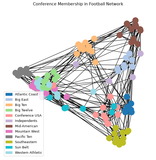

Conferences that overlap in this picture cannot be separated. With \(d = 3\) a third eigenvector becomes available to \(k\)-means, one we cannot see in the picture.

---

Spectral clustering with \(d = 3\), drawn in the \((\mathbf{w}_2, \mathbf{w}_3)\) layout. Cluster colours are arbitrary: compare the groupings.

compare_with_conferences(3)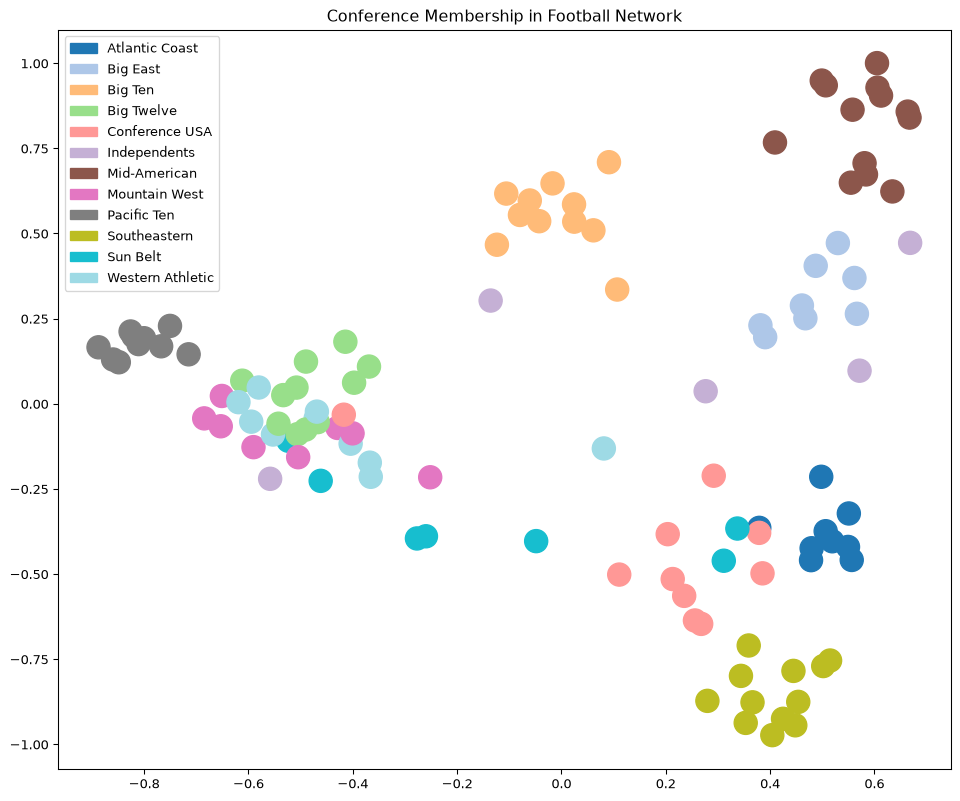

The third eigenvector separates groups that overlap in the two-dimensional picture.

Choosing \(d\) with the Adjusted Rand Index

from sklearn.metrics import adjusted_rand_score

dims = range(1, 15)
ari = [adjusted_rand_score(conf, spectral_clusters(d)) for d in dims]

plt.figure(figsize=(8, 4.5))
plt.plot(dims, ari, 'o-', color=OKABE_ITO[5])
plt.xlabel('Embedding dimension $d$ (number of eigenvectors)', size=14)
plt.ylabel('Adjusted Rand Index', size=14)
plt.title('Spectral clustering of the football network vs. conferences', size=14)
plt.ylim(0, 1)
plt.xticks(list(dims))
plt.grid(alpha=0.3)
plt.show()
best = int(np.argmax(ari))
print(f'ARI: d = 1: {ari[0]:.3f}, d = 2: {ari[1]:.3f}, d = 3: {ari[2]:.3f}, d = 6: {ari[5]:.3f}; '
      f'max {ari[best]:.3f} at d = {dims[best]}')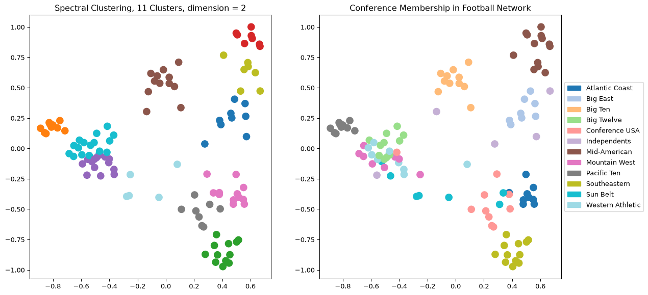

ARI: d = 1: 0.319, d = 2: 0.571, d = 3: 0.804, d = 6: 0.830; max 0.848 at d = 8

The ARI climbs steeply, from 0.32 with one eigenvector to 0.80 with three, then levels off: from \(d = 5\) on it stays between about 0.82 and 0.85 (the maximum, 0.848 at \(d = 8\), is barely above the 0.830 at \(d = 6\)). Extra eigenvectors neither help nor hurt much; the gain is in the first half-dozen.

The exact location of the maximum moves with the \(k\)-means seed (seeds 1 and 2 put it at \(d = 12\) and \(d = 6\)); the plateau does not. That is why we read the curve’s shape rather than its argmax.

Summary

• Three centralities, three notions of importance: closeness (reach, \(1/\sum_j d(i,j)\)), betweenness (brokerage, shortest paths through \(i\)), eigenvector (status, connected to the well-connected).
• Eigenvector centrality solves \(A\mathbf{x} = \lambda\mathbf{x}\) for the largest \(\lambda\); power iteration \(\mathbf{x} \leftarrow A\mathbf{x}/\Vert A\mathbf{x}\Vert\) computes it.
• Min cut peels off a leaf; the isoperimetric ratio \(\alpha\) divides by the smaller side and rewards balanced cuts.
• Laplacian \(L = D - A\), \(\mathbf{x}^TL\mathbf{x} = \sum_{(i,j)\in E}(x_i - x_j)^2\); the Fiedler vector \(\mathbf{w}_2\) is the smoothest non-constant assignment, and its sign, median or largest gap splits the graph.
• Spectral clustering: rows of \([\mathbf{w}_2, \dots, \mathbf{w}_{d+1}]\) as coordinates, then \(k\)-means; choose \(d\) by ARI when labels exist.

Before class, do the knowledge check. In class you will compute these centralities and run power iteration on a real network, build PageRank from scratch, and partition the network with its Fiedler vector.