Recap: Introduction to Networks
DS701 Session 23 — Mon Nov 23, 2026


Today’s plan
- 5 min — knowledge-check review
- 20 min — highlights and Q&A (answer or pass — answering always earns credit)
- 40 min — case study: mapping a nonprofit’s volunteer network
- wrap-up and cold-call check-ins
Knowledge-Check Review
KC 1: Degree, and why \(2e/n\)
An undirected graph has \(n\) nodes and \(e\) edges. State what the degree of a node is, and explain in one or two sentences why the average degree is \(2e/n\). Then say how the notion of degree changes for a directed graph.
KC 2: Clustering vs. short paths
The lecture defined a small-world network as one with high clustering and* short average path length. Explain why those two properties seem to be in tension (think of the ring lattice), and what Watts and Strogatz showed about how little it takes to get both at once.*
KC 3: Why compare to a random graph?
In the football example the lecture built a \(G(n,p)\) random graph with the same number of nodes and edges as the real network and compared the two. Why is a random graph a useful baseline, and name two ways the lecture showed real networks typically differ from \(G(n,p)\) — say what you would look at to see each difference.
Highlights
A graph is nodes + edges — and the adjacency matrix is the graph
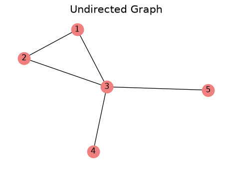
\(E = \{(1,2),(1,3),(2,3),(3,4),(3,5)\}\)
Number the nodes; \(A_{ij} = 1\) if \((i,j) \in E\), else \(0\):
\[ A = \begin{bmatrix} 0 & 1 & 1 & 0 & 0\\ 1 & 0 & 1 & 0 & 0\\ 1 & 1 & 0 & 1 & 1\\ 0 & 0 & 1 & 0 & 0\\ 0 & 0 & 1 & 0 & 0 \end{bmatrix} \qquad \text{row sums} = \begin{bmatrix} 2\\2\\4\\1\\1 \end{bmatrix} \]
- Edge list and \(A\) carry the same information — nothing is lost either way.
- Degree = row sum. Total \(= 10 = 2e\).
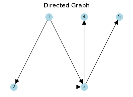
- Undirected \(\Leftrightarrow\) \(A\) symmetric. Directed: row \(i\) = out-edges, column \(j\) = in-edges — node 1 has in-degree 0, out-degree 2; node 3 has 2 and 2.
- Directed paths run head-to-tail: 1 → 3 → 5 exists, 5 → 1 does not. Reachability becomes one-way.
- Weighted: put the weight where the 1 was.
The first questions to ask of any network
- How big, how dense? \(n\) nodes, \(e\) edges, average degree \(2e/n\) (undirected).
- Who is connected to whom? Degree of each node — its distribution is the first summary.
- Is it connected? If not, list the connected components and work on the largest. (Directed: strongly connected components — mutual directed reachability.)
- How far apart are things? Shortest paths \(d(i,j)\); the diameter is the largest one, the average shortest path length \(L = \binom{N}{2}^{-1}\sum_{i<j} d(i,j)\) the typical one — both only make sense within a component.
- Do neighbours know each other? The clustering coefficient — next slide.
Every one of these is one NetworkX call: G.degree, nx.connected_components, nx.shortest_path_length, nx.diameter, nx.average_clustering. The skill is knowing which to ask, and what a surprising answer would look like.
The baseline: \(G(n,p)\)
- \(n\) nodes; each of the \(\binom{n}{2}\) pairs gets an edge independently with probability \(p\).
- Expected degree \(\langle k\rangle = p(n-1) \approx np\). Degrees are concentrated around \(np\) — no hubs.
- Clustering coefficient \(= p\): two of your neighbours are just two nodes.
- To match a real network with \(n\) nodes and \(e\) edges: \(p = e / \binom{n}{2}\).
It is not a model of anything real. It is what “no structure” looks like at this size and density — so anything the real graph does differently is worth explaining.
Real networks I: heavy tails
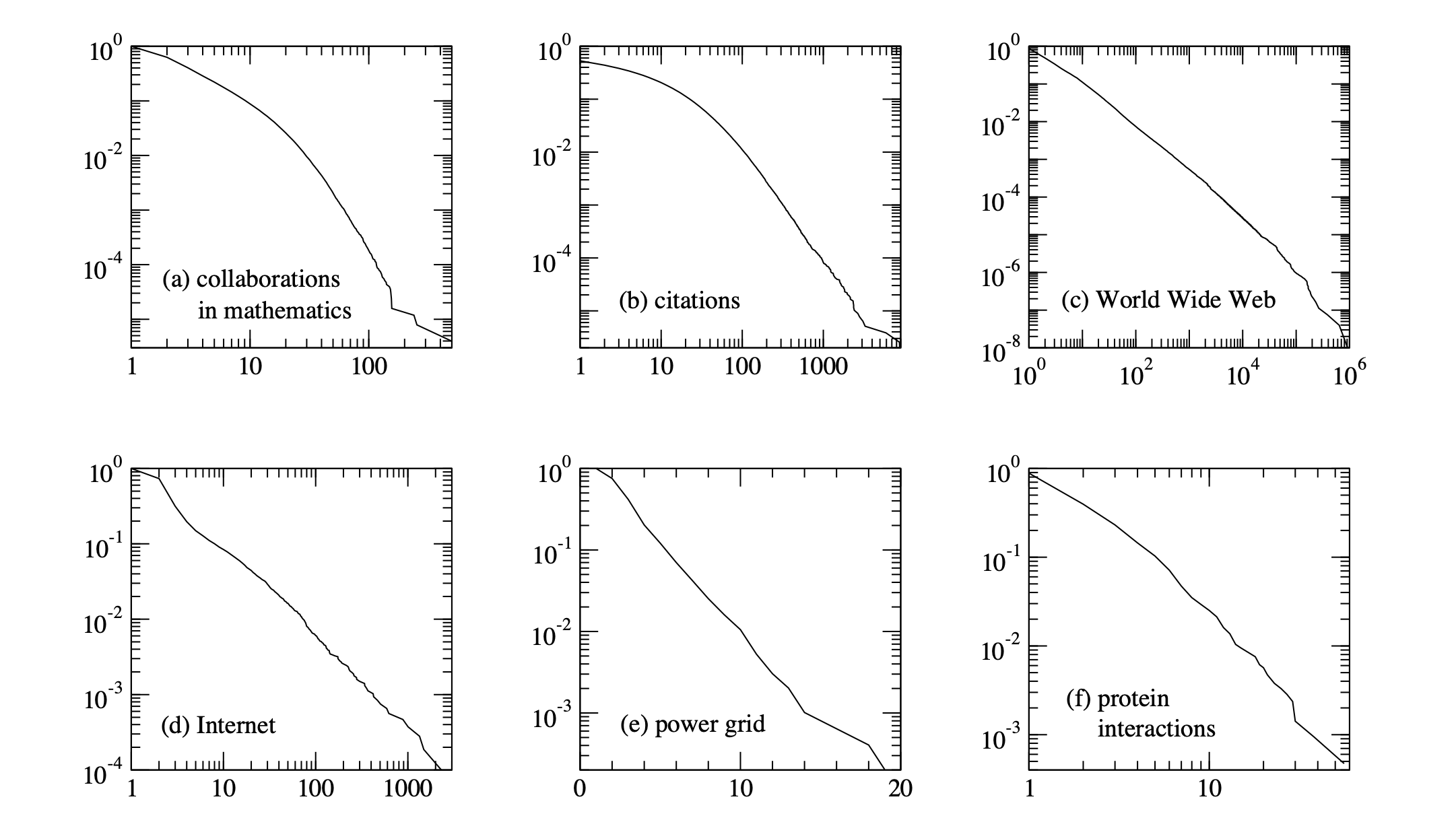
Degree distribution as a CCDF: \(P(X > x)\), the fraction of nodes with degree above \(x\).
- Power law / Pareto: \(P(X > x) = (k/x)^{\alpha}\) — a straight line on log–log axes, slope \(-\alpha\).
- Meaning: most nodes have few neighbours; a small but real set of nodes have very many. Hubs.
- \(G(n,p)\) with the same mean would show no such tail — its log–log CCDF falls off a cliff (lecture: Barabási–Albert max degree 100 vs. 13, both with mean degree 4).
- Not universal: the power grid (e) is straight on lin–log axes — an exponential tail.
Real networks II: clustering, and the small world
Clustering coefficient — the probability that two of your neighbours are connected.
\[ C^{(1)} = \frac{\sum_i \#\text{triangles at } i}{\sum_i \#\text{neighbour pairs at } i} \]
Five-node example: \(\dfrac{1+1+1}{1+1+6} = \dfrac{3}{8}\).
\(C^{(2)}\) averages the per-node ratios instead (nx.average_clustering): \(\dfrac{1}{5}\bigl(1+1+\tfrac16\bigr) = 0.433\).
Random graph: \(C = p\). Real networks: much higher.
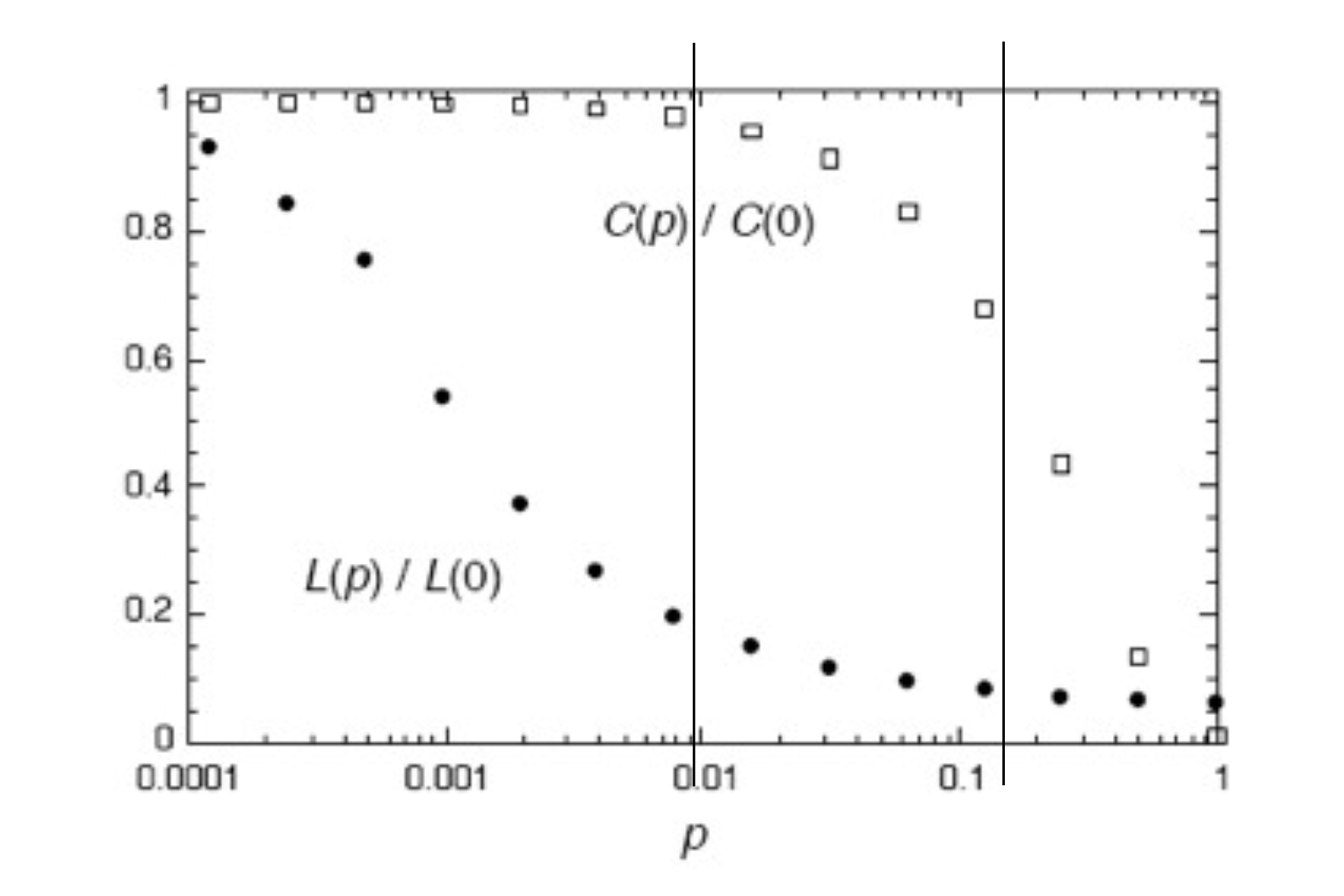
Watts–Strogatz: a few rewired edges collapse \(L\) while \(C\) holds. Small world = high clustering and short paths. Milgram’s letters arrived in about six links; Granovetter’s weak ties; Kevin Bacon is not special.
Putting it together: football vs. random
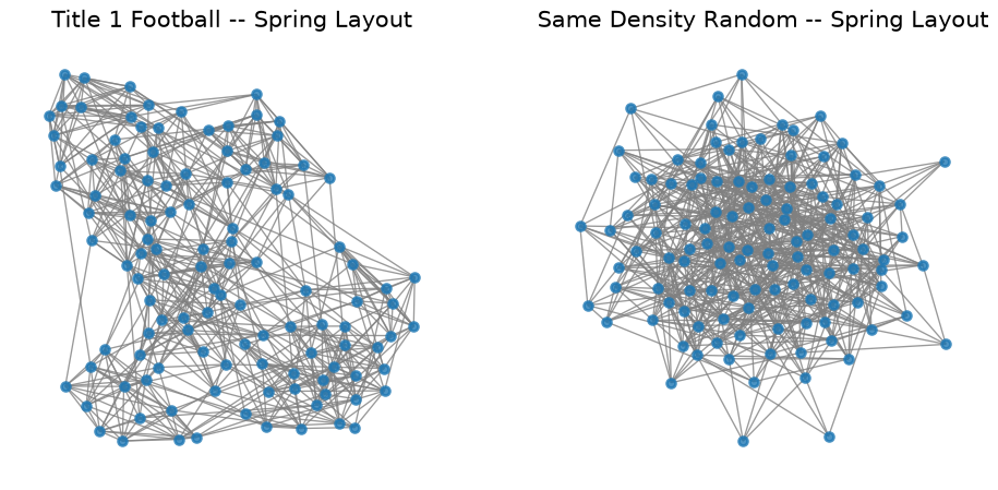
- Same \(n\), same \(e\). Coloured by conference: each clump is a conference; the random graph is a well-mixed blob.
- Clustering coefficient: real \(\gg\) random. Diameter and average path: both short.
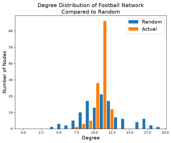
- Degree histogram: a spike at 11 games — a scheduling rule. “Different from random” here means more regular, not heavier-tailed. The baseline tells you that there is structure; you still have to say what.
Representation is a modelling choice
The same relationship data can be turned into several graphs — and they answer questions differently.
- Directed or undirected? “Follows” is directed; symmetrising it throws away who is followed vs. who follows. In-degree and out-degree rank people differently.
- Weighted or unweighted? Number of games played, strength of a tie, a distance. Shortest paths and “closest” nodes change when weights count.
- From a similarity matrix? Threshold last month’s distance matrix (L02) at \(\tau\): an edge where similarity \(> \tau\). Loose \(\tau\): one giant component. Tight \(\tau\): many islands. The components you find depend on a number you chose.
There is no representation-free “the network”. Today’s activity: same data, three representations, three sets of answers — then you decide which is right for the question. Next session: centrality and PageRank — the representation choice bites even harder there.
In-Class Activity
Activity — Case Study 20: Mapping a Volunteer Network for a Community Nonprofit
Goal: a community-services nonprofit has a volunteer shift log and no analyst; the board asks who works with whom, whether the volunteers are one community or several, and whether a few people hold it together. You prototype on Zachary’s karate club (ships with NetworkX; the real log awaits a privacy review): build the graph and its adjacency matrix (Part 1), components, paths and diameter against a \(G(n,p)\) baseline (Part 2), degree distributions — a heavy tail vs random (Part 3), and clustering vs random (Part 4) — then write the two-sentence memo, including which representation (plain, weighted, directed) the board’s questions actually need.
- Work in groups of 2–3. Open your section’s notebook.
- Parts marked (autograded) are submitted to Gradescope; the rest is participation.
- Staff will circulate — be ready to explain any part of your work.
- Dependencies:
numpy,pandas,matplotlib,scipy,networkx.


The activity notebook goes live on the day of the lecture. Colab is optional — you can also open it on GitHub and run it locally.
Going deeper
Full lecture notes: Introduction to Networks
- Graphs, Undirected and Directed Graphs — definitions and the five-node example
- Paths, Degree, Connectivity — reachability, in/out-degree, components and SCCs
- The Adjacency Matrix, walks via \(A^2\) and Density
- The \(G(n,p)\) Random Graph — the baseline and its average degree
- Degree Distributions, Power Laws and the empirical CCDF — Pareto, log–log axes, Barabási–Albert vs. \(G(n,p)\)
- Clustering and the worked calculation — \(C^{(1)}\) vs \(C^{(2)}\)
- Small Worlds — ring lattice, Milgram, Granovetter, Watts–Strogatz
- Visualizing Networks and Metrics — the football network vs. random
- Next: Centrality and Clustering