Recap: \(k\)-Nearest Neighbors, the Curse of Dimensionality, and Naive Bayes
DS701 Session 11 — Tue Oct 13, 2026 (Monday schedule)


Today’s plan
- 5 min — knowledge-check review
- 20 min — highlights and Q&A (answer or pass — answering always earns credit)
- 45 min — case study: which classifier should the consortium buy
- wrap-up and cold-call check-ins
Knowledge-Check Review
KC 1: What does \(k\)-NN actually do?
What happens at training vs. test time? Which hyperparameter sets complexity? Parametric or nonparametric?
Show answer
- Train: store the labeled data — the data is the model
- Test: distance to every stored point → \(k\) nearest → majority vote
- Knob: \(k\) — small = jagged, large = smooth
- although have to calculate distance to all \(n\) points each time
- but only need to find the \(k\) closest (e.g. maxheap versus full sort)
- Nonparametric: storage grows with the data
KC 2: What the curse does to “nearest”
Shell fraction \(f_d = 1-(1-\epsilon)^d \to 1\); min/avg pairwise distance \(\to 1\). What does this do to “nearest”, and why does it hurt \(k\)-NN?
Show answer
- The ball is nearly all shell — almost every point is at about the same distance from the center
- Closest point is barely closer than a typical one
- Distances concentrate → the \(k\) neighbours are a near-random handful
- Their labels say little about the query
- Fixing it needs exponentially many points (\(10^{40}\) bins for 40 features)
KC 3: Naive Bayes meets the curse
State the naive assumption. For \(d = 1{,}000\) binary word features, how many probabilities per class with vs. without it? Why might NB cope better than \(k\)-NN?
Show answer
- Assumption: \(P(x_1,\dots,x_d \mid C) = \prod_j P(x_j \mid C)\)
- Naive — words co-occur; but only the arg max must be right
- With: \(\approx 1{,}000\) per class · Without: \(2^{1000}\) per class
- NB never measures distance — data need grows linearly in \(d\)
- \(k\)-NN needs density — exponential in \(d\)
- Catch: one zero count kills the product → Laplace smoothing
This Lecture’s Big Ideas
Big Ideas
- \(k\)-NN: store the data, find the nearest neighbors
- \(k\) is the bias–variance knob
- Nonparametric model – the training data is the model
- suffers from the Curse of Dimensionality
- Curse of dimensionality: distances concentrate, data becomes sparse
- Accuracy is misleading for unbalanced data
- Naive Bayes: use Bayes’ rule
- Naive assumption: conditional independence
- Avoid zero probabilities with Laplace smoothing
Highlights
The data is the model
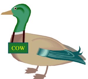
walks like a duck, quacks like a duck…
- Train: store the points. That’s it.
- Predict: distances → \(k\) closest → vote (hard) or vote fractions (soft)
- Nonparametric: the training set is the parameters
- Cost moves to test time: \(O(n)\) distances per prediction
- Scale your features — or one large-unit column picks the neighbours
\(k\) is the bias–variance knob
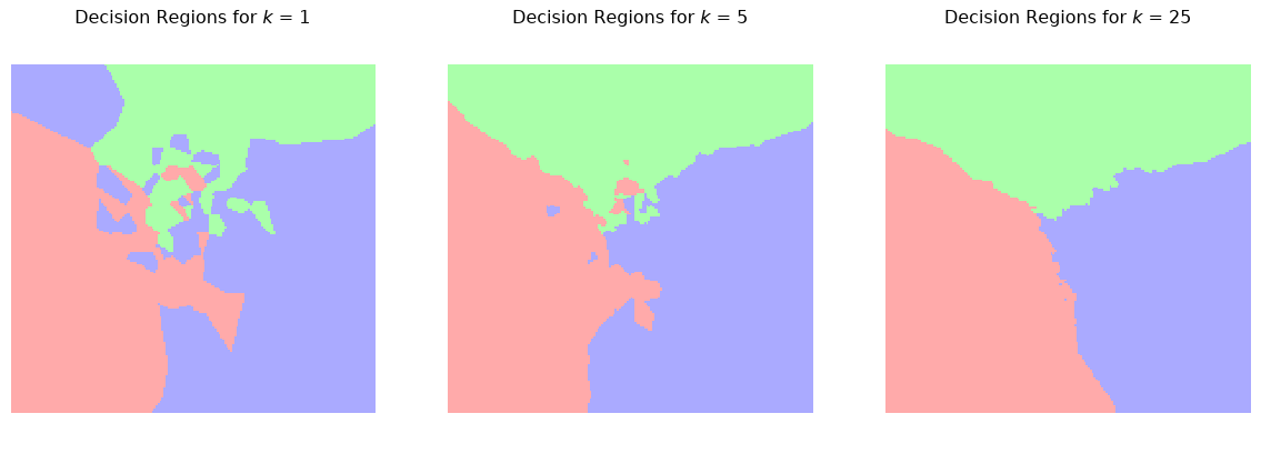
- \(k=1\): islands, 100% train accuracy — low bias, high variance
- \(k=25\): smooth regions — low variance, more bias
- Choose \(k\) on held-out data, never training error (lecture 07)
Choosing \(k\)
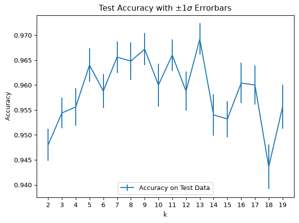
- Iris, mean of 50 random splits per \(k\)
- Peak at \(k = 13\), but error bars overlap 9–13
- One split = one noisy sample → average many, or use \(K\)-fold CV
- Tune on validation; touch test once
Accuracy is not the whole story
- Two-circles, 5-NN: 72% accuracy
- But only 14 of 28 Positives found
- Recall \(= TP/(TP+FN) = 50\%\)
- Precision \(= TP/(TP+FP) = 100\%\)
- 90/10 imbalance: “always majority” scores 90% and is useless
- Read the confusion matrix, not one number
The curse, part 1: space explodes
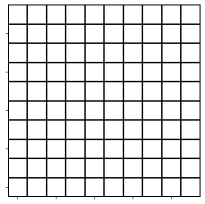
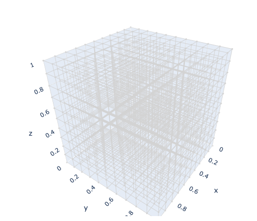
- \(k\)-NN needs dense data
- 10 bins × 40 features = \(10^{40}\) bins — nearly all empty
- Close in \(\mathbb{R}^d\) = close in every coordinate
- Data needed grows exponentially in \(d\)
The curse, part 2: “nearest” fades
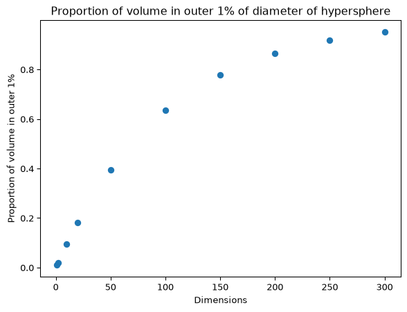

- Every neighbour is about equally far → \(k\) “nearest” ≈ random
- Fixes: other metrics (cosine), or reduce dimension (lectures 12–13)
Naive Bayes: classify with Bayes’ rule
\[ \hat{C} = \arg\max_{C_i} \; P(x_1\vert C_i) \cdot P(x_2\vert C_i) \cdots P(x_d\vert C_i)\,P(C_i) \]
- \(P(\mathbf{x})\) is the same for every class — drop it (MAP)
- Meningitis: evidence multiplies the prior by 15 → \(P(M \mid S) = 15 \times 10^{-4}\)
- Obstacle: the joint \(P(x_1,\dots,x_d \mid C_i)\) — \(10^{20}\) bins for 20 features
- assuming each feature can take one of 10 values
The naive assumption — and why it works
\[ P(x_1,\dots,x_d \mid C_i) = \prod_{j=1}^{d} P(x_j \mid C_i) \]
- \(10^{20}\) bins → \(20 \times 10\); training = counting
- Rarely true, but only the arg max must be right
- No distances → high \(d\) isn’t the same enemy
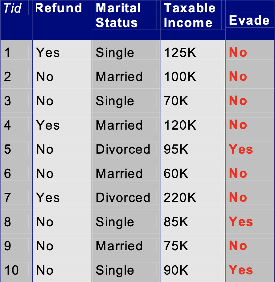
- One empty bin zeroes the product → Laplace smoothing
Going deeper
Full lecture notes: \(k\)-Nearest Neighbors, Curse of Dimensionality, and Naive Bayes
- Parametric vs. Nonparametric Models
- \(k\)-Nearest Neighbors · Varying \(k\) · Challenges for \(k\)-NN
- Curse: Points far apart · Distances concentrate · Outer shell · Example · Implications
- Precision and Recall · Confusion Matrix
- Choosing \(k\) on Validation Data · Hyperparameters: k-NN
- Naive Bayes — Bayes Rule · Naive Assumption · Worked Example · Laplace Smoothing · Dodging the Curse
- Background: Generalization — bias–variance, cross-validation
In-Class Activity
Case Study 09: Which classifier should the consortium buy?
- Client: the hospital consortium from Case Study 08
- They liked your depth-limited tree, but now:
- a \(k\)-NN vendor and a Naive Bayes vendor each claim to beat it
- one wants to sell 500 extra texture features
- Data: public Wisconsin diagnostic set (prototype — their own data isn’t released yet)
Your deliverables
- Scaling — does \(k\)-NN need standardized inputs?
- Choosing \(k\) — sweep \(k\), two metrics, cross-validate; how sure are you?
- Head-to-head vs. the tree — confusion matrix, precision & recall on malignant
- Explainability — Naive Bayes by hand on a toy table, with/without smoothing
- Memo — which model, one purchase condition, what 500 features do to “nearest”
Logistics
- Groups of 2–3 — open your section’s notebook
- (autograded) parts → Gradescope; the rest is participation
- Staff will circulate — be ready to explain your work


Goes live on lecture day. Colab optional — or run locally from GitHub.