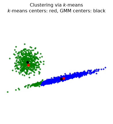
So far, we have seen how to cluster objects using \(k\)-means:
In \(k\)-means clustering every object is assigned to a single cluster.
This is called hard assignment.
And then we looked at hierarchical clustering:
In hierarchical clustering, objects are grouped into a tree of clusters.
Clusters are nested: each cluster is fully contained in the one above it.
However, there may be cases where we either cannot use hard assignments or we do not want to do it.
In particular, we might have reason to believe that the best description of the data is a set of overlapping clusters.
Overlapping Clusters
Income Level Example
Consider a population in terms of a simple binary income level: higher or lower than some threshold.
How might we model such a population in terms of the single feature age?
Income Level Sampling
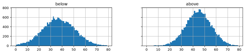
Let’s sample 20,000 above income threshold individuals and 20,000 below income threshold individuals.
From this sample we get have the following histograms.
Code
# original inspiration for this example from# https://www.cs.cmu.edu/~./awm/tutorials/gmm14.pdffrom scipy.stats import multivariate_normalnp.random.seed(4)df = pd.DataFrame(multivariate_normal.rvs(mean = np.array([37, 45]), cov = np.diag([196, 121]), size =20000), columns = ['below', 'above'])df.hist(bins =range(80), sharex =True, sharey=True, figsize=(12, 2))plt.show()
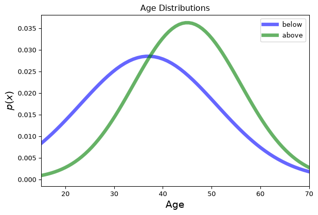
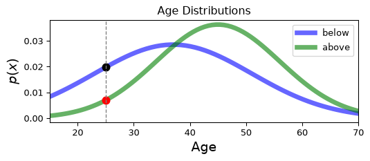
We find that ages of the below income threshold set have mean \(\mu=37\) with standard deviation \(\sigma=14\), while the ages of the above income threshold set have mean \(\mu=45\) with standard deviation \(\sigma=11\).
Income Level by Age
We can plot gaussian distributions for the two income levels.
Code
from scipy.stats import normplt.figure(figsize=(7, 4.5))x = np.linspace(norm.ppf(0.001, loc =37, scale =14), norm.ppf(0.999, loc =37, scale =14), 100)plt.plot(x, norm.pdf(x, loc =37, scale =14),'b-', lw =5, alpha =0.6, label ='below')x = np.linspace(norm.ppf(0.001, loc =45, scale =11), norm.ppf(0.999, loc =45, scale =11), 100)plt.plot(x, norm.pdf(x, loc =45, scale =11),'g-', lw =5, alpha =0.6, label ='above')plt.xlim([15, 70])plt.xlabel('Age', size=14)plt.legend(loc ='best')plt.title('Age Distributions')plt.ylabel(r'$p(x)$', size=14)plt.show()
Soft Clustering
two overlapping clusters.
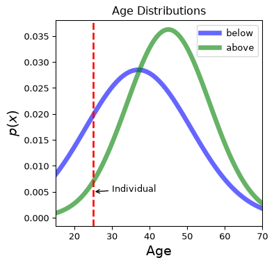
given some particular individual at a given age, say 25, we cannot say for sure which cluster they belong to.
use probability to quantify our uncertainty about cluster membership.
Individual belongs to the cluster 1 with some probability \(p_1\) and the cluster 2 with a different probability \(p_2\).
Naturally we expect the probabilities to sum up to 1.
This is called soft assignment, and a clustering using this principle is called soft clustering.
Conditional Probability
More formally, we say that an object can belong to each particular cluster with some probability, such that the sum of the probabilities adds up to 1 for each object.
For example, assuming that we have two clusters \(C_1\) and \(C_2\), we can have that an object \(x_1\) belongs to \(C_1\) with probability \(0.3\) and to \(C_2\) with probability \(0.7\).
Note that the distribution over \(C_1\) and \(C_2\) only refers to object \(x_1\).
A distribution is specified by its parameters \(\boldsymbol{\theta}\); for a Gaussian, \(\boldsymbol{\theta} = (\mu, \sigma^2)\).
The likelihood of i.i.d. samples \(x_1, \ldots, x_N\) is \(L(\boldsymbol{\theta}) = \prod_{n=1}^{N} p(x_n \vert \boldsymbol{\theta})\); the maximum likelihood estimate is the \(\boldsymbol{\theta}\) that maximizes it (equivalently, the log-likelihood \(\ell = \log L\)).
For a Gaussian, setting \(\nabla_{\mu}\ell = 0\) and \(\nabla_{\sigma}\ell = 0\) gives closed-form estimates:
Keep those two formulas in front of you – they reappear inside EM.
A GMM extends the single Gaussian to a mixture of \(K\) Gaussians, each with its own \(\boldsymbol{\mu}_k, \Sigma_k\) and a mixing weight \(\pi_k\).
We would like to estimate all of these by MLE, exactly as above.
But the mixture likelihood has a sum inside the log and no closed-form maximizer.
That is why we need the Expectation-Maximization (EM) algorithm – and, as we will see, its M-step is just the Gaussian MLE formulas, weighted by soft cluster assignments.
Gaussian Mixture Models
Univariate Gaussians
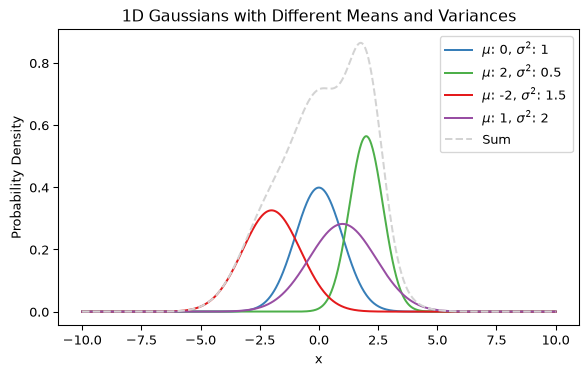
In GMMs we assume that each of our clusters follows a Gaussian (normal) distribution with their own parameters.
Code
import numpy as npimport matplotlib.pyplot as plt# Define the parameters for the 4 Gaussiansparams = [ {"mean": 0, "variance": 1, "color": "#377eb8"}, # Blue {"mean": 2, "variance": 0.5, "color": "#4daf4a"}, # Green {"mean": -2, "variance": 1.5, "color": "#e41a1c"}, # Red {"mean": 1, "variance": 2, "color": "#984ea3"} # Purple]# Generate x valuesx = np.linspace(-10, 10, 1000)total = np.zeros_like(x)plt.figure(figsize=(7, 4))# Plot each Gaussianfor param in params: mean = param["mean"] variance = param["variance"] color = param["color"]# Calculate the Gaussian y = (1/ np.sqrt(2* np.pi * variance)) * np.exp(- (x - mean)**2/ (2* variance))# Plot the Gaussian plt.plot(x, y, color=color, label=f"$\\mu$: {mean}, $\\sigma^2$: {variance}") total += yplt.plot(x, total, color="lightgray", linestyle="--", label="Sum")# Add legendplt.legend()# Add title and labelsplt.title("1D Gaussians with Different Means and Variances")plt.xlabel("x")plt.ylabel("Probability Density")# Show the plotplt.show()
This is a similar situation to our previous example where we considered labeling a person as above or below an income threshold based on the single feature age.
This could be a hypothetical situation with \(K=4\) normally distributed clusters.
Multivariate Gaussians
Given data points \(\mathbf{x}\in\mathbb{R}^{d}\), i.e., \(d\)-dimensional points, then we use the multivariate Gaussian to describe the clusters. The formula for the multivariate Gaussian is
where \(\Sigma\in\mathbb{R}^{d\times d}\) is the covariance matrix, \(\vert \Sigma\vert\), denote the determinant of \(\Sigma\), and \(\boldsymbol{\mu}\) is the \(d\)-dimensional vector of expected values.
The covariance matrix is the multidimensional analog of the variance. It determines the extent to which vector components are correlated.
See here for a refresher on the covariance matrix.
Notation
The notation \(x \sim \mathcal{N}(\mu, \sigma^2)\) is used to denote a univariate random variable that is normally distributed with expected value \(\mu\) and variance \(\sigma^{2}.\)
The notation \(\mathbf{x} \sim \mathcal{N}(\boldsymbol{\mu}, \Sigma)\) is used to denote a multivariate random variable that is normally distributed with mean \(\boldsymbol{\mu}\) and covariance matrix \(\Sigma\).
Multivariate Example: Cars
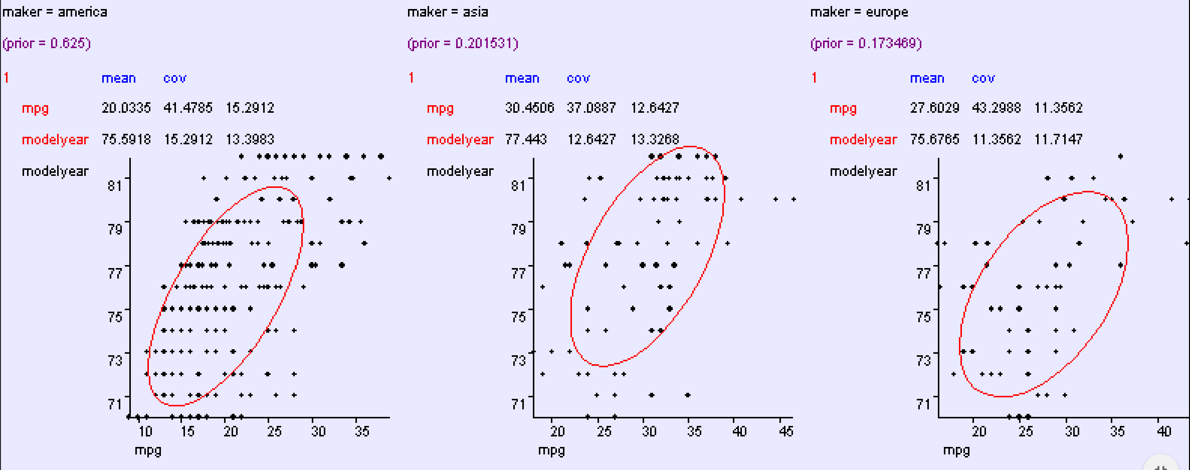
To illustrate a particular model, let us consider the properties of cars produced in the US, Europe, and Asia1.
For example, let’s say we are looking to classify cars based on their model year and miles per gallon (mpg).
It seems that the data can be described (roughly) as a mixture of threemultivariate Gaussian distributions.
Expectation-Maximization for Gaussian Mixture Models
The Gaussian Mixture Model
We observe \(n\) data points \(x_1, \ldots, x_n\) in \(\mathbb{R}^d\) that appear to come from \(K\) clusters.
A Gaussian Mixture Model (GMM) assumes each data point is generated by the following process:
Choose a cluster \(k \in \{1, 2, \ldots, K\}\) with probability \(\pi_k\) (where \(\sum_{k=1}^K \pi_k = 1\))
Generate the point from that cluster’s Gaussian: \(x_i \sim \mathcal{N}(\mu_k, \Sigma_k)\)
The probability density of observing point \(x_i\) is:
In Probabilistic Modeling the log turned a product into a sum of simple terms, and the derivative of each term gave a closed-form estimate.
Here there is a sum inside the log. The terms do not separate.
Setting the gradient to zero gives a system of coupled equations with no closed-form solution.
EM in One Slide
Let \(z_i \in \{1, \ldots, K\}\) be the cluster that generated \(x_i\). We never observe it: \(z_i\) is a latent variable.
If we knew every \(z_i\), estimating \(\theta\) would be lecture 05 again: \(\mu_k\) is the mean of the points in cluster \(k\), \(\Sigma_k\) their covariance, \(\pi_k\) their fraction of the data.
If we knew \(\theta\), we could compute how probable each cluster is for each point. That is Bayes’ rule.
We know neither. This is a classic 🐓 and 🥚 problem.
Expectation-Maximization (EM) breaks the loop by alternating:
E-step: with the current \(\theta\), compute \(\gamma_{ik} = P(z_i = k \mid x_i, \theta)\) for every point and every cluster. This is a soft assignment.
M-step: treat the \(\gamma_{ik}\) as fractional memberships and re-estimate \(\theta\) with the lecture-05 formulas, weighted.
Each round can only increase \(\ell(\theta)\), so the iteration converges (to a local maximum).
Let’s do the E-step by hand for a single point first.
Bayes’ Rule for One Point
Back to the income example, this time with the parameters known:
black = norm.pdf(25, loc=37, scale=14) # density under 'below'red = norm.pdf(25, loc=45, scale=11) # density under 'above'p_above = red *0.5/ (black *0.5+ red *0.5)print(f'P(above | age 25) = {p_above:.3f}, P(below | age 25) = {1- p_above:.3f}')
P(above | age 25) = 0.260, P(below | age 25) = 0.740
So this 25-year-old belongs to “above” with probability 0.26 and to “below” with probability 0.74. That pair of numbers is a soft assignment.
In EM notation it is one row of the responsibilities: \(\gamma_{i,\text{above}} = 0.26\) and \(\gamma_{i,\text{below}} = 0.74\).
E-Step: Compute Responsibilities
You just computed one entry. The E-step does this for every point \(i\) and every cluster \(k\), using the current parameters \(\theta^{(t)}\):
Compare with the MLE formulas from lecture 05: same sample mean and sample covariance, except that every point contributes to every cluster, weighted by how responsible that cluster is for it.
If every \(\gamma_{ik}\) were exactly 0 or 1, these collapse to per-cluster means and covariances. That is the \(k\)-means update.
Watch It Run
Let’s implement EM from scratch for the 1-D age data. The whole algorithm is three short functions.
Code
ages = np.r_[df['below'], df['above']] # 40,000 ages; the labels are thrown awaydef e_step(x, pi, mu, sigma):# responsibilities: n x K, each row sums to 1 dens = np.column_stack([pi[k] * norm.pdf(x, mu[k], sigma[k]) for k inrange(len(pi))])return dens / dens.sum(axis=1, keepdims=True)def m_step(x, gamma):# weighted MLE: the lecture-05 formulas with responsibilities as weights N_k = gamma.sum(axis=0) pi = N_k /len(x) mu = (gamma * x[:, None]).sum(axis=0) / N_k sigma = np.sqrt((gamma * (x[:, None] - mu)**2).sum(axis=0) / N_k)return pi, mu, sigmadef log_likelihood(x, pi, mu, sigma): mixture =sum(pi[k] * norm.pdf(x, mu[k], sigma[k]) for k inrange(len(pi)))return np.log(mixture).sum()
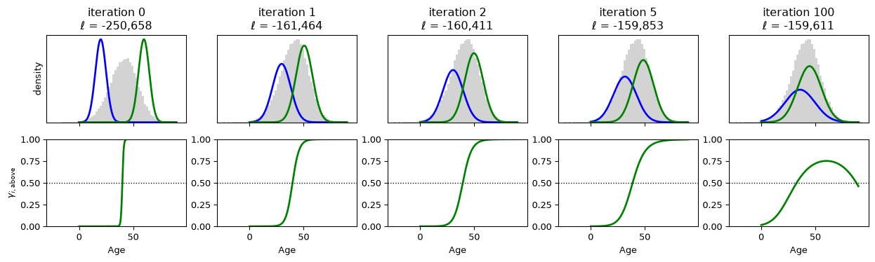
Start from deliberately bad guesses: clusters far too narrow and far too far apart.
Top row: the two weighted components \(\pi_k \mathcal{N}(x \mid \mu_k, \sigma_k^2)\) (blue, green) over a histogram (gray) of the data. Bottom row: the responsibility \(\gamma_{i,\text{above}}\) as a function of age.
The first iteration does most of the work: the components jump to the data and the soft boundary moves to where the two curves cross.
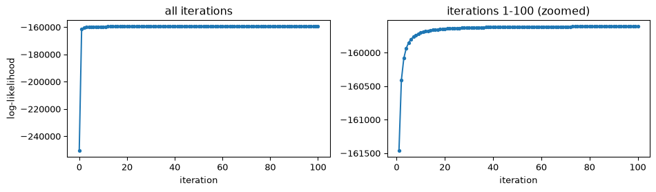
After that the changes are small. The log-likelihood never decreases.
By iteration 100 the boundary is no longer a single cutoff: the wider “below” Gaussian wins back the oldest ages from the narrower “above” one. A soft assignment captures that; a threshold on age cannot.
Watch It Run, cont.
Code
lls = [h[3] for h in history]fig, ax = plt.subplots(1, 2, figsize=(10, 3))ax[0].plot(lls, 'o-', ms=3)ax[0].set_xlabel('iteration'); ax[0].set_ylabel('log-likelihood'); ax[0].set_title('all iterations')ax[1].plot(range(1, 101), lls[1:], 'o-', ms=3)ax[1].set_xlabel('iteration'); ax[1].set_title('iterations 1-100 (zoomed)')plt.tight_layout()plt.show()
EM after 100 iterations: pi=[0.42 0.58], mu=[35.9 44.7], sigma=[13.9 11.1],  ll=-159,611.4
Generating parameters:   pi=[0.5 0.5], mu=[37 45], sigma=[14 11],  ll=-159,614.1
EM’s parameters have a slightly higher likelihood than the ones that generated the data, yet they are not the same. Two Gaussians that overlap this much are hard to tell apart even with 40,000 samples: many nearby mixtures fit almost equally well, so the likelihood is nearly flat and EM crawls along it.
Keep this in mind for the overlapping-clusters example later.
Initialization
Initialize the \(K\) means \(\mu_k\) randomly, or with \(k\)-means (sklearn’s default, init_params='kmeans')
Initialize covariances \(\Sigma_k\), often as identity matrices or the sample covariance
Initialize mixing weights \(\pi_k = \frac{1}{K}\)
EM finds a local maximum, so the result depends on this choice. In practice you run several initializations and keep the one with the highest log-likelihood (n_init in sklearn).
Iteration and Convergence
Alternate E and M steps. The log-likelihood is guaranteed not to decrease, so monitor it and stop when it stops moving:
Log-likelihood:\(\lvert \ell^{(t)} - \ell^{(t-1)} \rvert < \text{tol}\), with \(\text{tol}\) small (e.g. \(10^{-4}\)), or
Parameters:\(\lVert \theta^{(t)} - \theta^{(t-1)} \rVert_2 < \text{tol}\), and always
Iteration cap:\(t > \text{max\_iterations}\) (e.g. 100), for cases that converge slowly or never fully stabilize.
The tolerance matters. On the age data above, sklearn’s default tolerance stops after about 8 iterations, well inside the flat region.
Why Does Alternating Work?
The algorithm above is what everyone implements. Here is what each step is doing to the likelihood, and where the closed-form updates come from.
If the assignments \(z_i\) were known, the complete-data log-likelihood would be
There is no sum inside the log: it separates by cluster and maximizes in closed form.
E-step: we don’t know \(\mathbb{1}(z_i = k)\), so we replace it with its expected value under the current parameters, \(\mathbb{E}\!\left[\mathbb{1}(z_i = k) \mid x_i, \theta^{(t)}\right] = P(z_i = k \mid x_i, \theta^{(t)}) = \gamma_{ik}\).
M-step: maximize the resulting expected complete-data log-likelihood. The \(\gamma_{ik}\) are constants in it, so the maximizer is exactly the weighted MLE formulas.
Updating \(\pi_k\) requires a division (given \(N_k\))
k-means vs GMMs
Let’s pause for a minute and compare GMM/EM with \(k\)-means.
GMM/EM
Initialize randomly or using some rule
Compute the probability that each point belongs in each cluster
Update the clusters (weights, means, and variances).
Repeat 2-3 until convergence.
\(k\)-means
Initialize randomly or using some rule
Assign each point to a single cluster
Update the clusters (means).
Repeat 2-3 until convergence.
From a practical standpoint, the main difference is that in GMMs, data points do not belong to a single cluster, but have some probability of belonging to each cluster.
In other words, as stated previously, GMMs use soft assignment.
For that reason, GMMs are also sometimes called soft \(k\)-means.
However, there is also an important conceptual difference.
The GMM starts by making an explicit assumption about how the data were generated.
It says: “the data came from a collection of multivariate Gaussians.”
We made no such assumption when we came up with the \(k\)-means problem. In that case, we simply defined an objective function and declared that it was a good one.
Nonetheless, it appears that we were making a sort of Gaussian assumption when we formulated the \(k\)-means objective function. However, it wasn’t explicitly stated.
The point is that because the GMM makes its assumptions explicit, we can
examine them and think about whether they are valid, and
replace them with different assumptions if we wish.
For example, it is perfectly valid to replace the Gaussian assumption with some other probability distribution. As long as we can estimate the parameters of such distributions from data (e.g., have MLEs), we can use EM in that case as well.
Versatility of EM
A final statement about EM generally. EM is a versatile algorithm that can be used in many other settings. What is the main idea behind it?
Notice that the problem definition only required that we find the clusters, i.e., the \((\pi_k, \mu_k, \Sigma_k)\).
However, the EM algorithm posited that we should find as well the \(P(z_i = k \mid x_i) = \gamma_{ik}\), the probability that each point is a member of each cluster.
This is the true heart of what EM does.
By adding variables to the problem, the latent \(z_i\) and their posteriors \(\gamma_{ik}\), it finds a way to make the problem solvable.
Those latent variables don’t show up in the final answer.
Examples
Example 1
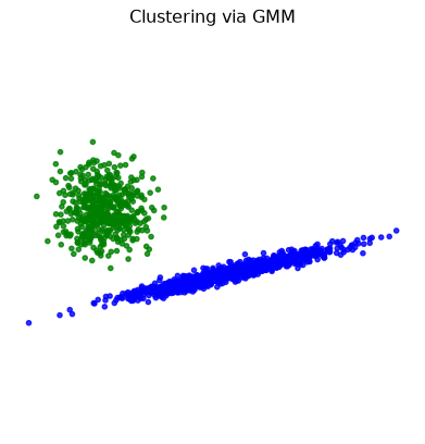
sklearn’s GaussianMixture runs exactly the E- and M-steps we just wrote, in \(d\) dimensions with full covariance matrices \(\Sigma_k\). Here is an example using GMM.
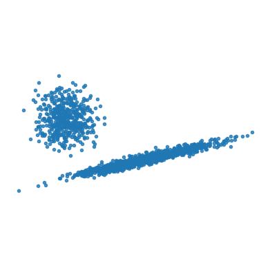
We’re going to create two clusters, one spherical, and one highly skewed.
Code
# Number of samples of larger componentn_samples =1000# C is a transfomation that will make a heavily skewed 2-D GaussianC = np.array([[0.1, -0.1], [1.7, .4]])print(f'The covariance matrix of our skewed cluster will be:\n{C.T@C}')
The covariance matrix of our skewed cluster will be:
 [[2.9  0.67]
 [0.67 0.17]]
Code
import warningswarnings.filterwarnings('ignore')rng = np.random.default_rng(0)# now we construct a data matrix that has n_samples from the skewed distribution,# and n_samples/2 from a symmetric distribution offset to position (-4, 2)X = np.r_[(rng.standard_normal((n_samples, 2)) @ C),.7* rng.standard_normal((n_samples//2, 2)) + np.array([-4, 2])]
Code
plt.figure(figsize=(5, 5))plt.scatter(X[:, 0], X[:, 1], s =10, alpha =0.8)plt.axis('equal')plt.axis('off')plt.show()
Code
# Fit a mixture of Gaussians with EM using two componentsimport sklearn.mixturegmm = sklearn.mixture.GaussianMixture(n_components=2, covariance_type='full', init_params ='kmeans')y_pred = gmm.fit_predict(X)
Code
plt.figure(figsize=(5, 5))colors = ['bg'[p] for p in y_pred]plt.title('Clustering via GMM')plt.axis('off')plt.axis('equal')plt.scatter(X[:, 0], X[:, 1], color = colors, s =10, alpha =0.8)plt.show()
Code
for clus inrange(2):print(f'Cluster {clus}:')print(f' weight: {gmm.weights_[clus]:0.3f}')print(f' mean: {gmm.means_[clus]}')print(f' cov: \n{gmm.covariances_[clus]}\n')
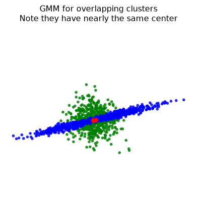
plt.figure(figsize=(5, 5))colors = ['bgrky'[p] for p in y_pred_over]plt.title('GMM for overlapping clusters\nNote they have nearly the same center')plt.scatter(X[:, 0], X[:, 1], color = colors, s =10, alpha =0.8)plt.axis('equal')plt.axis('off')plt.plot(gmm.means_[:,0], gmm.means_[:,1], 'ro')plt.show()
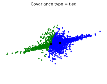
plt.figure(figsize=(5.5, 4))colors = ['bgrky'[p] for p in y_pred]plt.scatter(X[:, 0], X[:, 1], color=colors, s=10, alpha=0.8)plt.title('Covariance type = tied')plt.axis('equal')plt.axis('off')plt.plot(gmm.means_[:,0],gmm.means_[:,1], 'ok')plt.show()
Non-Skewed Clusters
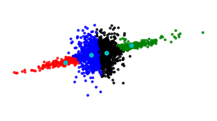
Perhaps you believe in even more restricted shapes: all clusters should have their axes aligned with the coordinate axes.
That is, clusters are not skewed.
Then you only need to estimate the diagonals of the covariance matrices - just \(Kd\) parameters.
This is specified by the GMM parameter covariance_type='diag'.
plt.figure(figsize=(5.5, 3))colors = ['bgrky'[p] for p in y_pred]plt.scatter(X[:, 0], X[:, 1], color = colors, s =10, alpha =0.8)plt.axis('equal')plt.axis('off')plt.plot(gmm.means_[:,0], gmm.means_[:,1], 'oc')plt.show()
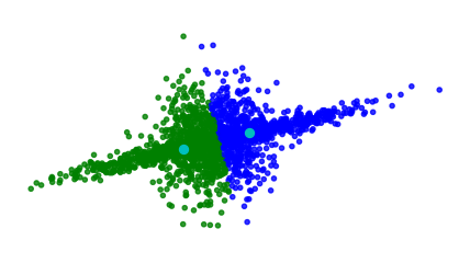
Round Clusters
Finally, if you believe that all clusters should be round, then you only need to estimate the \(K\) variances.
This is specified by the GMM parameter covariance_type='spherical'.
plt.figure(figsize=(5.5, 3))colors = ['bgrky'[p] for p in y_pred]plt.scatter(X[:, 0], X[:, 1], color = colors, s =10, alpha =0.8)plt.axis('equal')plt.axis('off')plt.plot(gmm.means_[:,0], gmm.means_[:,1], 'oc')plt.show()