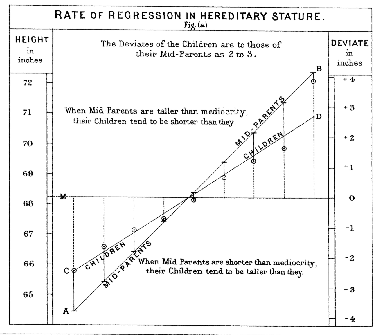
In 1886 Francis Galton published his observations about the height of children compared to their parents.
Regression to the Mean
Defined mid-parent as the average of the heights of the parents.
When parents are taller or shorter than average, their children are more likely to be closer to the average height than their parents.
So called “regression to the mean.”
Galton fit a straight line to this effect, and the fitting of lines or curves to data has come to be called regression as well.
Praise versus Punishment
Daniel Kahneman
In the 60s, psychologist Daniel Kahneman studied the effect of praise versus punishment on performance of Israeli Air Force trainees. He was led to believe that praise was more effective than punishment.
Air force trainers disagreed and said that when they praised pilots that did well, they usually did worse the next time, and when they punished pilots that did poorly, they usually did better the next time.
What Kahneman later realised was that this phenomenon could be explained by the idea of regression to the mean.
If a pilot does worse than average on a task, they are more likely to do better the next time, and if they do better than average, they are more likely to do worse the next time.
Is it a good strategy to fire a coach after a bad season?
bad season -> fire and replace coach -> better season next year
When this could be interpreted as:
bad season (outlier) -> regression to the mean -> better season next year
This applies to many situations
“I had so many colds last year, and then I started herbal remedies, and I have much fewer colds this year.”
“My investments were doing quite bad last year, so switched investment managers, and now it is doing much better.”
“The team had a terrible season, so we fired the coach – and this year they’re winning again.”
When in fact, they could be (at least partially) explained by:
Regression to the mean
The praise-versus-punishment and coaching stories above are two famous instances; Kahneman’s version is in Thinking, Fast and Slow. We will meet the effect once more at the end of this lecture, where it falls out of the algebra of least squares.
Model Types
The most common form of machine learning is regression, which means constructing an equation that describes the relationships among variables.
It is a form of supervised learning:
whereas classification deals with predicting categorical features (labels or classes),
regression deals with predicting continuous features (real values).
Fit to Linear Models
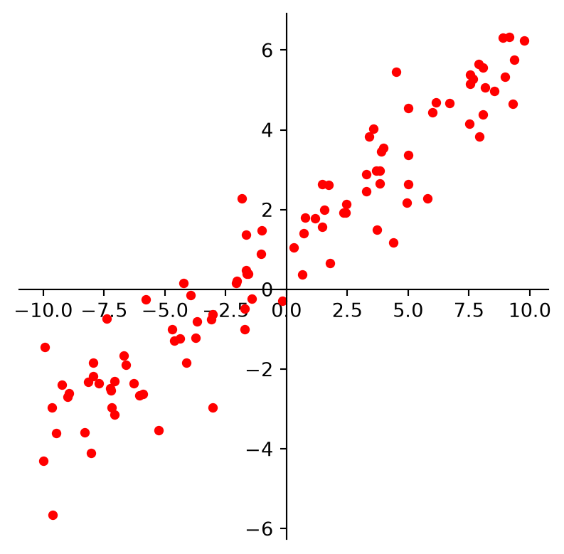
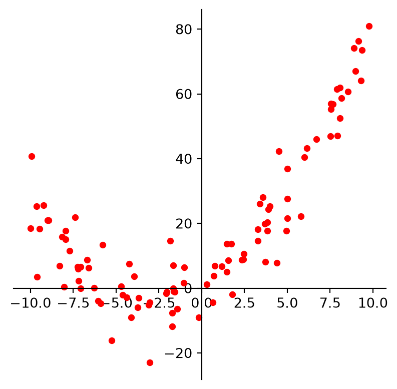
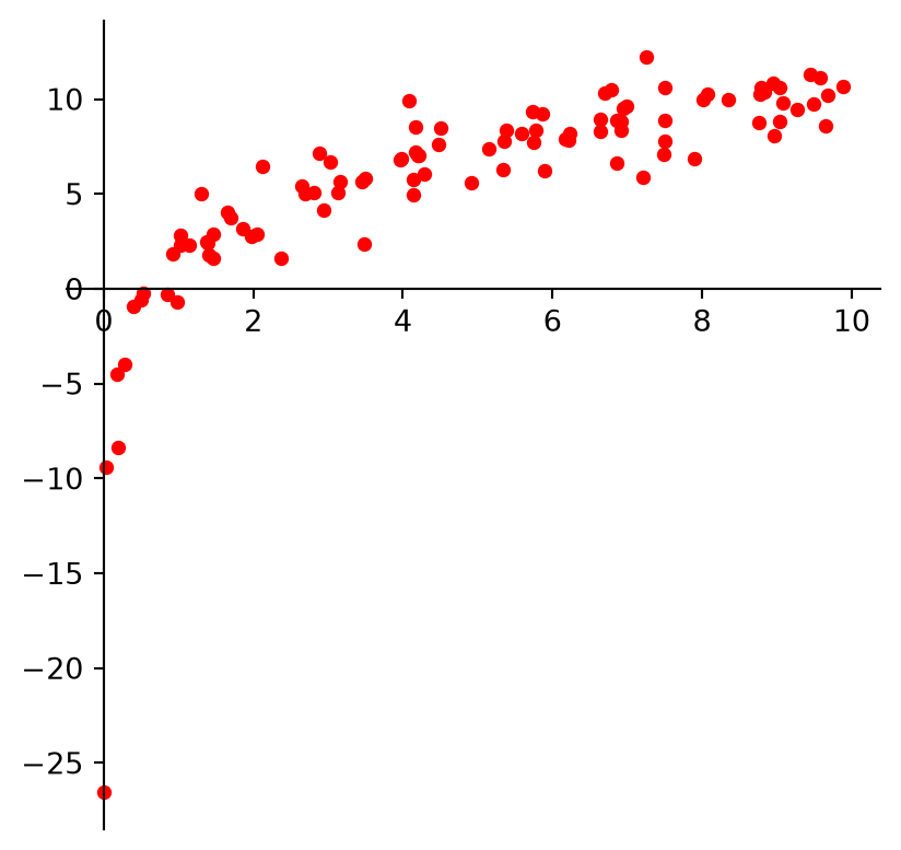
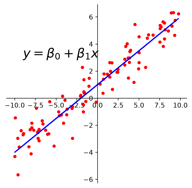
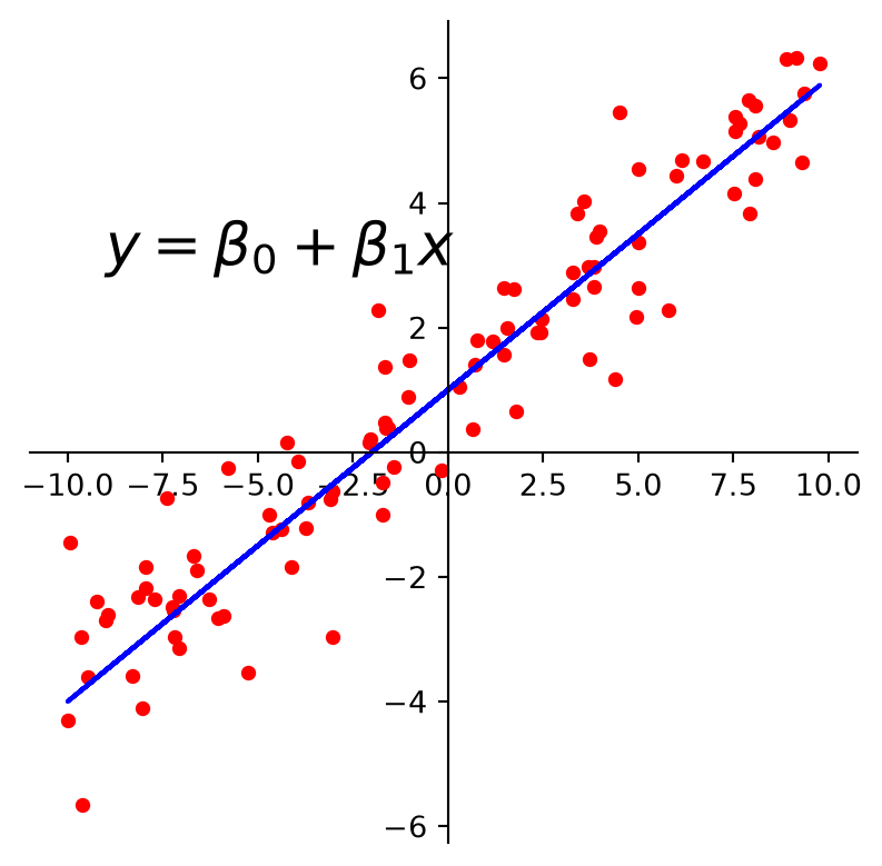
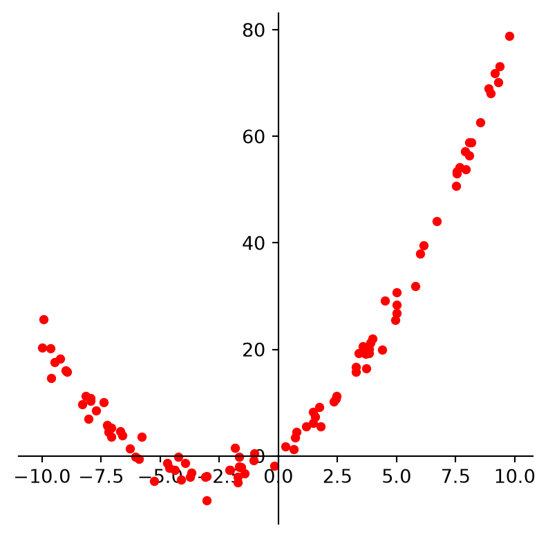
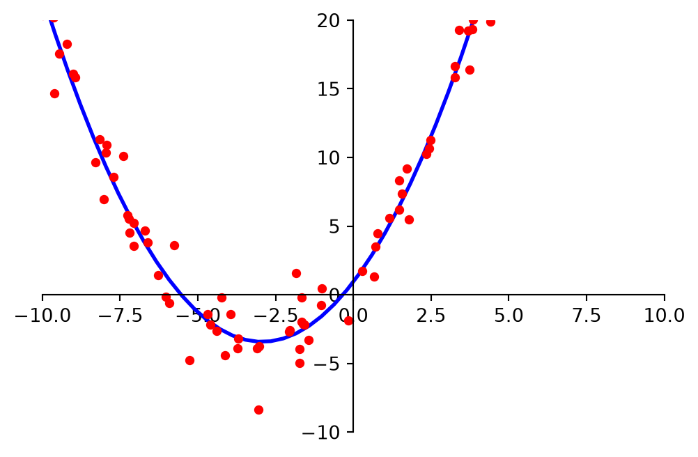
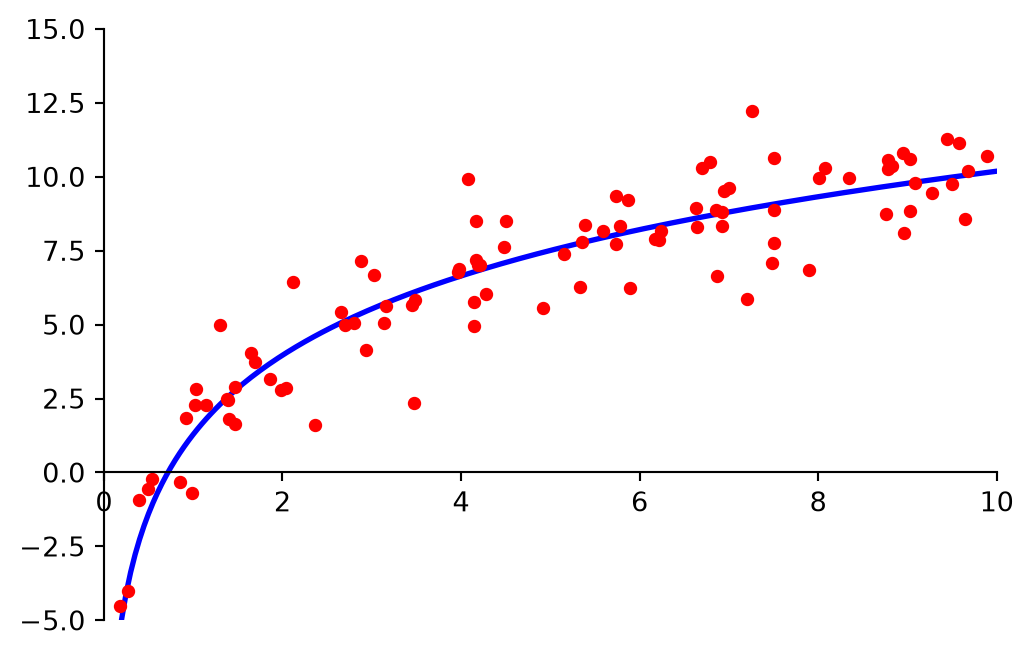
For example, we may look at these points and decide to model them using a line.
Clearly, none of these datasets agrees perfectly with the proposed model.
So the question arises:
How do we find the best linear function (or quadratic function, or logarithmic function) given the data?
Framework
Framework
This problem has been studied extensively in the field of statistics.
Certain terminology is used:
Some values are referred to as “independent,” and
Some values are referred to as “dependent.”
The basic regression task is:
given a set of independent variables
and the associated dependent variables,
estimate the parameters of a model (such as a line, parabola, etc) that describes how the dependent variables are related to the independent variables.
The independent variables are collected into a matrix \(X,\) sometimes called the design matrix.
The dependent variables are collected into an observation vector \(\mathbf{y}.\)
The parameters of the model (for any kind of model) are collected into a parameter vector \(\boldsymbol\beta.\)
Of course, if the data points don’t actually lie exactly on a line,
… then there are no parameters \(\beta_0, \beta_1\) for which the predicted \(y\)-values in \(X\boldsymbol\beta\) equal the observed \(y\)-values in \(\mathbf{y}\),
… and \(X\boldsymbol\beta=\mathbf{y}\) has no solution.
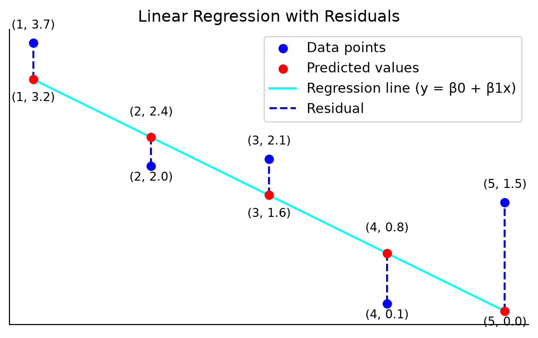
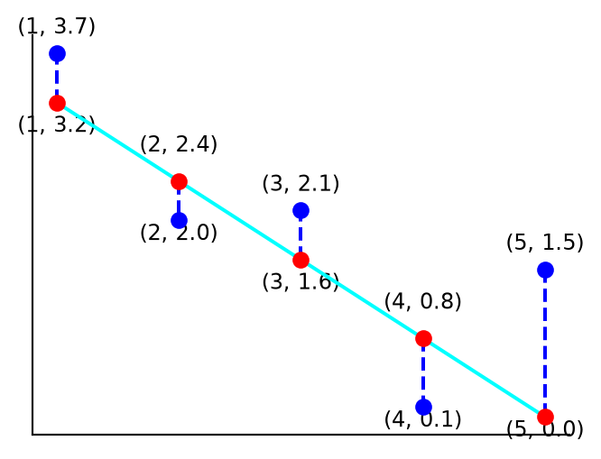
Now, since the data doesn’t fall exactly on a line, we have decided to seek the \(\boldsymbol\beta\) that minimizes the sum of squared residuals, i.e.,
The sum of squares of the residuals is exactly the square of the distance between the vectors \(X\boldsymbol\beta\) and \(\mathbf{y}.\)
Computing the least-squares solution of \(X\boldsymbol\beta = \mathbf{y}\) is equivalent to finding the \(\boldsymbol\beta\) that determines the least-squares line.
Now, to obtain the least-squares line, find the least-squares solution to \(X\boldsymbol\beta = \mathbf{y}.\)
Where does that solution come from? Not from a formula to memorize – from a picture.
TipPrerequisites
The next two slides use the column space of a matrix, orthogonal projection, and the normal equations. If these are rusty, read Least squares in the linear-algebra refresher first; its Least squares beware page is also worth a look before you write np.linalg.inv(X.T @ X) yourself.
Least squares is a projection
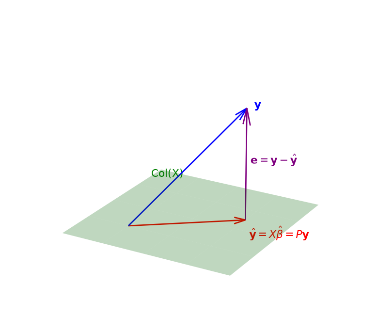
As \(\boldsymbol\beta\) varies, \(X\boldsymbol\beta\) ranges over the column space\(\text{Col}(X)\): all linear combinations of the columns of \(X\).
We want the point \(\hat{\mathbf{y}} = X\hat{\boldsymbol\beta}\) of \(\text{Col}(X)\) that is closest to \(\mathbf{y}\).
The closest point of a subspace is the orthogonal projection of \(\mathbf{y}\) onto it. So the residual \(\mathbf{e} = \mathbf{y} - \hat{\mathbf{y}}\) is perpendicular to the subspace, hence to every column of \(X\): \[X^T(\mathbf{y} - X\hat{\boldsymbol\beta}) = \mathbf{0}.\]
The same condition from calculus
The loss is the squared length of the residual, \(\lVert \mathbf{y} - X\boldsymbol\beta \rVert^2\). Its gradient is
The geometry says why it holds; the derivative gives an equation to solve. It is a minimum, not just a flat point, because the loss is a convex bowl.
Rearranging \(X^T(\mathbf{y} - X\hat{\boldsymbol\beta}) = \mathbf{0}\) gives the normal equations:
\[
X^TX\hat{\boldsymbol\beta} = X^T\mathbf{y}.
\]
They say exactly this: the residual \(X\hat{\boldsymbol\beta} - \mathbf{y}\) is normal (i.e. orthogonal) to the column space of \(X\).
The normal equations always have at least one solution (\(X^T\mathbf{y}\) lies in the column space of \(X^T\), which equals the column space of \(X^TX\)).
If \(X^TX\) is invertible, the solution is unique:
\(P = X(X^TX)^{-1}X^T\) is the projection matrix, or hat matrix (it puts the hat on \(\mathbf{y}\)). It depends only on \(X\), not on \(\mathbf{y}\).
\(P\) is symmetric (\(P^T = P\)) and idempotent (\(P^2 = P\)): projecting twice changes nothing.
\(\operatorname{tr} P = p\), the number of columns of \(X\): the fit “uses up” \(p\) degrees of freedom.
The residual is \(\mathbf{e} = (I - P)\mathbf{y}\), and \(\hat{\mathbf{y}}^T\mathbf{e} = \mathbf{y}^TP(I-P)\mathbf{y} = 0\): fitted values and residuals are orthogonal. That is Pythagoras, \(\|\mathbf{y}\|^2 = \|\hat{\mathbf{y}}\|^2 + \|\mathbf{e}\|^2\), and it becomes \(\text{TSS} = \text{RSS} + \text{ESS}\) below.
The diagonal entry \(P_{ii}\) is the leverage of observation \(i\): how hard \(y_i\) pulls on its own fitted value. It returns when we look at residuals.
When is \(X^TX\) invertible?
For \(X\) an \(n \times p\) matrix (\(n\) observations, \(p\) columns):
\[
X^TX \text{ is invertible} \iff X \text{ has full column rank, i.e. } \operatorname{rank}(X) = p,
\]
meaning no column of \(X\) is a linear combination of the others.
This requires \(n \geq p\) (at least as many observations as columns), but \(n \ge p\) alone is not enough: two identical columns make \(X^TX\) singular at any \(n\).
When \(X^TX\) is singular the normal equations still have solutions – infinitely many. The fitted values \(\hat{\mathbf{y}} = P\mathbf{y}\) are still unique (the projection is), but the coefficients are not: the fit is determined, \(\boldsymbol\beta\) is not. Nearly collinear columns cause the same trouble in a milder form, which is where regularization comes in next lecture.
The General Linear Model
The General Linear Model
Another way that the inconsistent (i.e. no exact solution) linear system is often written is to collect all the residuals into a residual vector.
where \(\boldsymbol\epsilon\) is the residual vector.
Any equation of this form is referred to as a linear model.
In this formulation, the goal is to find the \(\boldsymbol\beta\) so as to minimize the norm of \(\boldsymbol\epsilon\), i.e., \(\Vert\boldsymbol\epsilon\Vert.\)
In some cases, one would like to fit data points with something other than a straight line.
In cases like this, the matrix equation is still \(X\boldsymbol\beta = \mathbf{y}\), but the specific form of \(X\) changes from one problem to the next.
Least-Squares Fitting of Other Models
In model fitting, the parameters of the model are what is unknown.
A central question for us is whether the model is linear in its parameters.
For example, is this model linear in its parameters?
\[
y = \beta_0 e^{-\beta_1 x}
\]
It is not linear in its parameters.
Is this model linear in its parameters?
\[
y = \beta_0 e^{-2 x}
\]
It is linear in its parameters.
For a model that is linear in its parameters, an observation is a linear combination of (arbitrary) known functions.
In other words, a model that is linear in its parameters is
np.linalg.inv(X.T @ X) @ X.T @ y mirrors the formula and is fine for a first look, but forming the inverse is numerically unstable when columns of \(X\) are nearly collinear – small rounding errors in \(X^TX\) become large errors in \(\hat{\boldsymbol\beta}\). From here on we use np.linalg.lstsq(X, y), which solves the same least-squares problem stably (via a QR or SVD factorization); np.linalg.solve(X.T @ X, X.T @ y) is the other common choice.
The refresher’s Least squares beware page has a three-line example where the inverse gets the answer wrong, and Lecture 11B shows what near-collinearity does to the coefficients.
with \(f_0,\dots,f_{p-1}\) any sort of known functions and \(\beta_0,\dots,\beta_{p-1}\) unknown weights.
Example
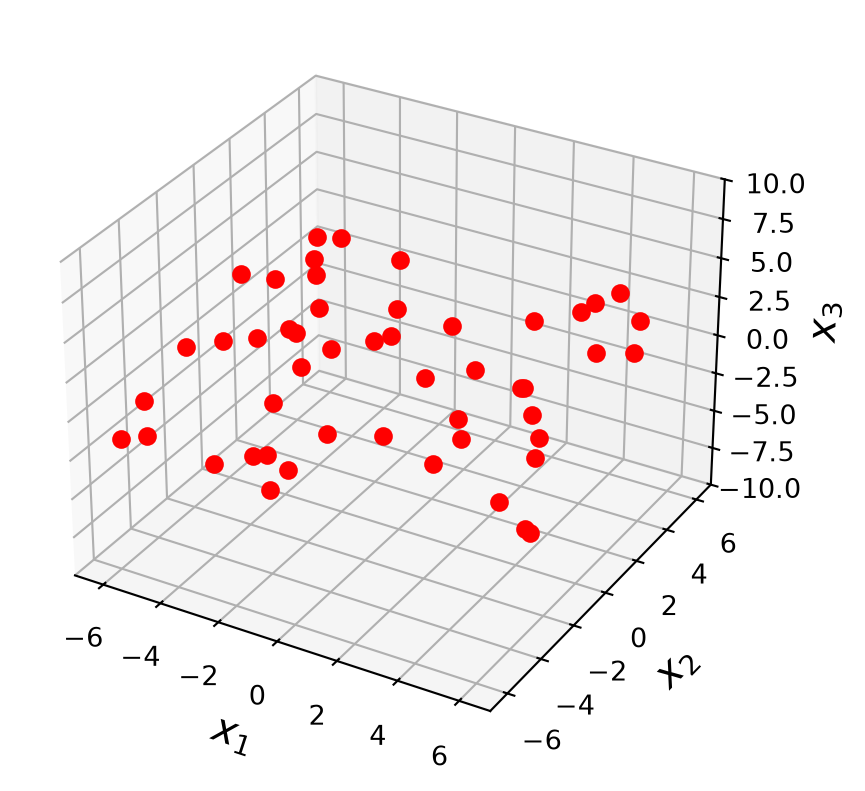
Let’s take an example. Here are a set of points in \(\mathbb{R}^3\):
Code
ax = ut.plotSetup3d(-7, 7, -7, 7, -10, 10, figsize = (5, 5))v = [4.0, 4.0, 2.0]u = [-4.0, 3.0, 1.0]npts =50# set locations of points that fall within x,ynp.random.seed(1)xc =-7.0+14.0* np.random.random(npts)yc =-7.0+14.0* np.random.random(npts)A = np.array([u,v]).T# project these points onto the planeP = A @ np.linalg.inv(A.T @ A) @ A.Tcoords = P @ np.array([xc, yc, np.zeros(npts)])coords[2] += np.random.randn(npts)ax.plot(coords[0], coords[1], 'ro', zs=coords[2], markersize =6)plt.show()
Example
In geography, local models of terrain are constructed from data
\[
(u_1, v_1, z_1), \dots, (u_n, v_n, z_n),
\]
where \(u_j, v_j\), and \(z_j\) are latitude, longitude, and altitude, respectively.
Let’s describe the linear models that gives a least-squares fit to such data.
The solution is called the least-squares plane.
Solution
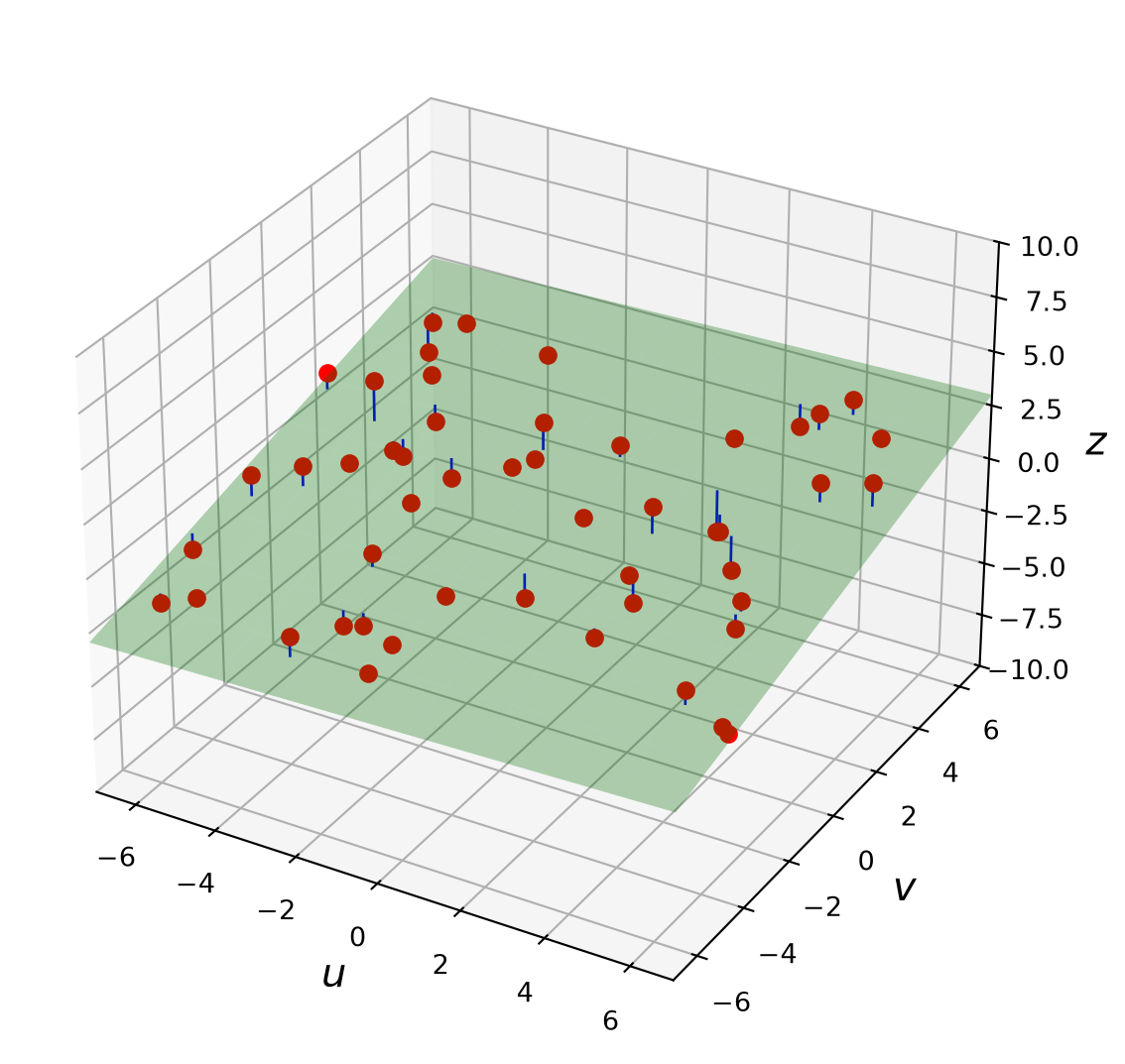
The model is \(z = \beta_0 + \beta_1 u + \beta_2 v + \epsilon\): altitude as a linear function of latitude and longitude. We expect the data to satisfy these equations:
u_obs, v_obs, z_obs = coords# design matrix [1, u, v] and the least-squares planeX_plane = np.column_stack([np.ones(npts), u_obs, v_obs])beta_plane, *_ = np.linalg.lstsq(X_plane, z_obs, rcond=None)z_hat = X_plane @ beta_planeax = ut.plotSetup3d(-7, 7, -7, 7, -10, 10, figsize = (7, 7))ax.set_xlabel('$u$', size=15)ax.set_ylabel('$v$', size=15)ax.set_zlabel('$z$', size=15)# the fitted plane ...uu, vv = np.meshgrid(np.linspace(-7, 7, 10), np.linspace(-7, 7, 10))ax.plot_surface(uu, vv, beta_plane[0] + beta_plane[1] * uu + beta_plane[2] * vv, color='green', alpha=0.3)# ... and the residual from each point to itfor ui, vi, zi, zh inzip(u_obs, v_obs, z_obs, z_hat): ax.plot([ui, ui], [vi, vi], [zi, zh], 'b-', lw=1)ax.plot(u_obs, v_obs, 'ro', zs=z_obs, markersize=6)plt.show()
The green surface is the fitted plane \(\hat z = \hat\beta_0 + \hat\beta_1 u + \hat\beta_2 v\); the blue segments are the residuals it minimizes (in the sum of squares).
This example shows that the linear model for multiple regression has the same form as the model for the simple regression in the earlier examples.
We can see that the general principle is the same across all the different kinds of linear models.
Once \(X\) is defined properly, the normal equations for \(\boldsymbol\beta\) have the same matrix form, no matter how many variables are involved.
Thus, for any linear model where \(X^TX\) is invertible, the least squares estimate is
As a result, \(0\leq R^2\leq 1\) – on the training data, for a model with an intercept. That is what makes \(\text{TSS} = \text{RSS} + \text{ESS}\) hold.
Computed on held-out data (e.g. validation or test) (as r2_score does for Ames below) RSS can exceed TSS, and \(R^2\) can be negative: the model predicts worse than the constant \(\overline{y}\).
This is more specifically called the centered\(R^2\); it assumes an intercept. We will meet the uncentered variant in a moment, when a software package quietly switches to it.
The closer the value of \(R^2\) is to \(1\) the better the fit of the regression:
small values of RSS imply that the residuals are small and therefore we have a better fit.
\(R^2\) is called the coefficient of determination.
It tells us “how well does the model predict the data?”
\(R^2\) and Pearson’s \(r\)
\(R^2\) is related to, but not the same thing as, Pearson’s correlation coefficient\(r\).
For simple regression (one feature plus an intercept), \(R^2 = r^2\) exactly, where \(r = \text{corr}(x, y)\). That is where the notation comes from, and why people sometimes write \(r^2\).
In general (any number of features, with an intercept, in-sample), \[R^2 = \text{corr}(\mathbf{y}, \hat{\mathbf{y}})^2,\] the squared correlation between the observations and the model’s predictions.
So \(R^2\) is a correlation squared, but between \(\mathbf{y}\) and \(\hat{\mathbf{y}}\), not between two raw variables. Two features can each be correlated with \(y\) while the model built from them predicts it poorly; to judge predictions against ground truth, use \(R^2\) (and use it on held-out data).
OLS in Practice
OLS in Practice
First, we’ll look at a test case on synthetic data. We’ll use Scikit-Learn’s make_regression function.
from sklearn import datasetsX, y = datasets.make_regression(n_samples=100, n_features=20, n_informative=5, bias=0.1, noise=30, random_state=1)
And then use the statsmodels package to fit the model.
import statsmodels.api as sm# statsmodels does not add an intercept for you: prepend a column of onesX_with_intercept = sm.add_constant(X)model = sm.OLS(y, X_with_intercept)results = model.fit()
The \(R^2\) value is very good. We can see that the linear model does a very good job of predicting the observations \(y_i\).
NoteUncentered \(R^2\)
sm.OLS does not add an intercept for you – hence sm.add_constant. Fit sm.OLS(y, X) on the raw X instead and the summary switches to the uncentered\(R^2\),
and says so in a footnote. Without a constant column the residuals need not sum to zero, \(\text{TSS} = \text{RSS} + \text{ESS}\) fails and the centered \(R^2\) can be negative, so statsmodels divides by \(\sum y_i^2\) instead of \(\sum (y_i - \overline{y})^2\). The uncentered number is almost always larger and is not comparable to the centered one. Try it.
Aside: Summary Statistics
Here is what all the statistics in the summary table mean. Throughout, \(n\) is the number of observations and \(p\) the number of columns of \(X\)including the constant (so \(p = 21\) above). When the model has no constant, statsmodels reports the uncentered versions of the first three statistics (see the callout above), with \(p\) in place of \(p - 1\).
R-squared:
Definition: the fraction of the variance of the dependent variable explained by the model – the centered \(R^2\) defined above.
where \(y_i\) is the actual value, and \(\hat{y}_i\) is the predicted value from the regression.
Interpretation: Higher values (closer to 1) indicate a better in-sample fit. It never decreases when a column is added, so it cannot by itself choose between models.
Adjusted R-squared:
Definition: Adjusts \(R^2\) for the number of columns in the model, so that adding a useless column is penalized rather than rewarded.
Interpretation: It is a more conservative measure of fit than the regular \(R^2\), particularly useful when comparing models with different numbers of predictors. Unlike \(R^2\), it can fall when a column is added.
F-statistic:
Definition: The F-statistic tests whether the overall regression model is significant, i.e., whether at least one of the (non-intercept) predictors explains a significant amount of the variance in the dependent variable.
Interpretation: A high F-statistic suggests that the model is statistically significant.
Prob (F-statistic):
Definition: This is the p-value associated with the F-statistic. It indicates the probability that the observed F-statistic would occur if the null hypothesis (that none of the predictors are significant) were true.
Interpretation: A small p-value (typically less than 0.05) suggests that the model is statistically significant, meaning that at least one predictor is important.
Log-Likelihood:
Definition: The log-likelihood measures the likelihood that the model could have produced the observed data. It is a measure of the fit of the model to the data.
where \(\sigma^2\) is the variance of the residuals.
Interpretation: A higher log-likelihood indicates a better fit of the model.
Akaike Information Criterion (AIC):
Definition: AIC is a measure of the relative quality of a statistical model for a given set of data. It penalizes the likelihood function for adding too many parameters.
where \(p\) is the number of parameters, and \(\mathcal{L}\) is the log-likelihood.
Interpretation: Lower AIC values suggest a better model fit, but it penalizes for overfitting.
Bayesian Information Criterion (BIC):
Definition: Similar to AIC, BIC penalizes models with more parameters, but more strongly than AIC. It is used to select among models.
Formula: \(\text{BIC} = p \log(n) - 2 \log(\mathcal{L})\)
where \(p\) is the number of parameters, \(n\) is the number of observations, and \(\mathcal{L}\) is the log-likelihood.
Interpretation: A lower BIC indicates a better model, with stronger penalties for models with more parameters.
Coefficient Table:
The first two columns are the independent variables and their coefficients. It is the \(m\) in \(y = mx + b\). One unit of change in the variable will affect the variable’s coefficient’s worth of change in the dependent variable, with the other variables held fixed. If the coefficient is negative, they have an inverse relationship. As one rises, the other falls.
The std error is an estimate of the standard deviation of the coefficient, a measurement of the amount of variation in the coefficient throughout its data points.
The t is related and is a measurement of the precision with which the coefficient was measured. A low std error compared to a high coefficient produces a high t statistic, which signifies a high significance for your coefficient.
P>|t| is one of the most important statistics in the summary. It uses the t statistic to produce the P value: the probability of seeing a t statistic at least this extreme if the true coefficient were zero. For example, a P value of 0.378 says that, if the variable had no effect on the dependent variable, a coefficient this far from zero would still appear 37.8% of the time by chance. It is not the probability that the variable has no effect. Proper model analysis will compare the P value to a previously established alpha value, or a threshold with which we can apply significance to our coefficient. A common alpha is 0.05, which few of our variables pass in this instance.
[0.025 and 0.975] are the lower and upper ends of the 95% confidence interval for the coefficient, roughly the estimate plus or minus two standard errors. If the interval contains zero, the data cannot distinguish the coefficient from zero.
The coefficient description came from this blog post which also describes the other statistics in the summary table.
Back to the example.
Some of the independent variables may not contribute to the accuracy of the prediction.
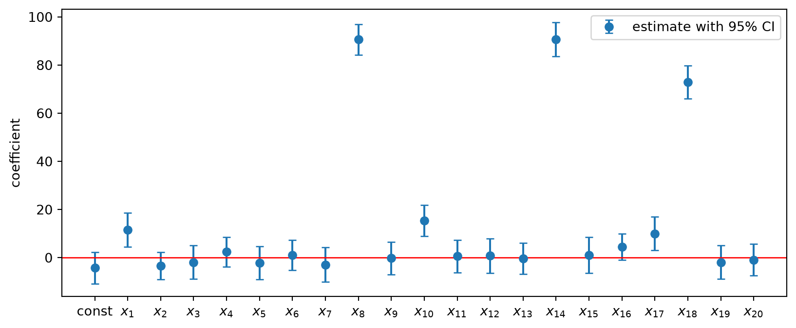
Each coefficient comes with a 95% confidence interval – the [0.025 0.975] columns of the table. Plotting them side by side makes the table readable at a glance:
If a coefficient’s interval contains zero, the data cannot distinguish it from zero, and we cannot assume that there is any relationship between that independent variable and the observations. Six intervals sit clearly away from zero – but make_regression was told n_informative=5. One of the six is a false positive: at the 95% level, roughly one useless column in twenty will look significant by chance, and we have fifteen useless columns.
Confidence Interval Formula
For coefficient \(\beta_j\), the 95% confidence interval is:
where: - \(\hat{\beta}_j\) is the estimated coefficient - \(t_{\alpha/2, n-p}\) is the critical value from the t-distribution with \(n-p\) degrees of freedom (for 95% CI, \(\alpha = 0.05\)) - \(\text{SE}(\hat{\beta}_j)\) is the standard error of \(\hat{\beta}_j\)
Calculating the Standard Error
The standard errors come from the variance-covariance matrix of the coefficient estimates:
This is a \(p \times p\) matrix where: - Diagonal elements are variances of each coefficient - Off-diagonal elements are covariances between coefficients
The standard error is the square root of the \(j\)-th diagonal element of the variance-covariance matrix.
Interpretation
In the statsmodels summary, the [0.025, 0.975] columns are exactly these bounds: - Lower bound: \(\hat{\beta}_j - t_{0.025, n-p} \cdot \text{SE}(\hat{\beta}_j)\) - Upper bound: \(\hat{\beta}_j + t_{0.025, n-p} \cdot \text{SE}(\hat{\beta}_j)\)
If this interval contains zero, the coefficient is not statistically significant - we can’t distinguish it from no effect.
Why \((X^T X)^{-1}\)?
This matrix captures the geometry of your design: - Larger values → more uncertainty (wider CIs) - Happens when: features are correlated (multicollinearity) or you have fewer data points
In other words, if the confidence interval for the parameter includes zero, the associated independent variable may not have any predictive value.
Here that is nearly harmless – make_regression built \(y\) from five informative columns, and we kept those five plus one impostor. In general, though, be careful: choosing the features and judging the fit on the same data is the Lecture 7 anti-pattern. The refit looks better than it is, because the selection step already used the noise in this sample (that is exactly how the impostor got in).
The honest version checks the smaller model on data it has not seen – which is exactly what we do for the Ames houses next.
Dropping a column is also an all-or-nothing choice. Next lecture’s regularization replaces manual pruning with a penalty that shrinks coefficients toward zero smoothly, and lets held-out data pick how hard to shrink.
Real Data: House Prices in Ames, Iowa
Let’s see how powerful multiple regression can be on a real-world example.
A typical application of linear models is predicting house prices.
Linear models have been used for this problem for decades, and when a municipality does a value assessment on your house, they typically use a linear model.
We can consider various measurable attributes of a house (its “features”) as the independent variables, and the most recent sale price of the house as the dependent variable.
For our case study, we will use the features:
Lot Area (sq ft),
Gross Living Area (sq ft),
Number of Fireplaces,
Number of Full Baths,
Number of Half Baths,
Garage Area (sq ft),
Basement Area (sq ft)
So our design matrix will have 8 columns (including the constant for the intercept):
\[
X\beta = \mathbf{y},
\]
and it will have one row for each house in the data set, with \(y\) the sale price of the house.
We will use data from housing sales in Ames, Iowa from 2006 to 2009:
import os, urllib.requestdef data_file(path):"""Course data file: use a local copy (here, or in the repo root above a notebook in jupyter_notebooks/), else fetch it from the Materials repo (Colab)."""for prefix in ('', '../'):if os.path.exists(prefix + path):return prefix + path os.makedirs(os.path.dirname(path) or'.', exist_ok=True) urllib.request.urlretrieve('https://raw.githubusercontent.com/tools4ds/DS701-Materials-FA26/main/'+ path, path)return pathdf = pd.read_csv(data_file('data/ames-housing-data/train.csv'))
Note that removing the intercept will cause the \(R^2\) to go up, which is counter-intuitive. The reason is explained here – but amounts to the fact that the formula for \(R^2\) with/without an intercept is different.
Let’s split the data into training and test sets.
Code
from sklearn import utils, model_selectionX_train, X_test, y_train, y_test = model_selection.train_test_split( X_intercept, y, test_size =0.5, random_state =0)
Fit the model to the training data.
Code
model = sm.OLS(y_train, X_train)results = model.fit()print(results.summary())
                            OLS Regression Results
==============================================================================
Dep. Variable:                      y   R-squared:                       0.759
Model:                            OLS   Adj. R-squared:                  0.757
Method:                 Least Squares   F-statistic:                     325.5
Date:                Fri, 16 Oct 2026   Prob (F-statistic):          1.74e-218
Time:                        15:17:15   Log-Likelihood:                -8746.5
No. Observations:                 730   AIC:                         1.751e+04
Df Residuals:                     722   BIC:                         1.755e+04
Df Model:                           7
Covariance Type:            nonrobust
===============================================================================
                  coef    std err          t      P>|t|      [0.025      0.975]
-------------------------------------------------------------------------------
const       -4.285e+04   5350.784     -8.007      0.000   -5.34e+04   -3.23e+04
LotArea         0.2361      0.131      1.798      0.073      -0.022       0.494
GrLivArea      48.0865      4.459     10.783      0.000      39.332      56.841
Fireplaces   1.089e+04   2596.751      4.192      0.000    5787.515     1.6e+04
FullBath      1.49e+04   3528.456      4.224      0.000    7977.691    2.18e+04
HalfBath      1.56e+04   3421.558      4.559      0.000    8882.381    2.23e+04
GarageArea     98.9856      8.815     11.229      0.000      81.680     116.291
TotalBsmtSF    62.6392      4.318     14.508      0.000      54.163      71.116
==============================================================================
Omnibus:                      144.283   Durbin-Watson:                   1.937
Prob(Omnibus):                  0.000   Jarque-Bera (JB):              917.665
Skew:                           0.718   Prob(JB):                    5.39e-200
Kurtosis:                       8.302   Cond. No.                     6.08e+04
==============================================================================

Notes:
[1] Standard Errors assume that the covariance matrix of the errors is correctly specified.
[2] The condition number is large, 6.08e+04. This might indicate that there are
strong multicollinearity or other numerical problems.
We see that we have:
\(\beta_0\): Intercept of -$42,850
\(\beta_1\): Marginal value of one square foot of Lot Area: $0.23
but NOTICE - this coefficient is not statistically different from zero!
\(\beta_2\): Marginal value of one square foot of Gross Living Area: $48
\(\beta_3\): Marginal value of one additional fireplace: $10,890
\(\beta_4\): Marginal value of one additional full bath: $14,900
\(\beta_5\): Marginal value of one additional half bath: $15,600
\(\beta_6\): Marginal value of one square foot of Garage Area: $99
\(\beta_7\): Marginal value of one square foot of Basement Area: $62
Why is a half bath ($15,600) worth more than a full bath ($14,900)?
Each \(\beta_j\) holds the other six features fixed: \(\beta_5\) is the value of a half bath given the living area, basement, garage and so on.
Half baths co-occur with bigger, newer houses, and the coefficient absorbs some of what those features do not capture. Add or remove a correlated feature and the other coefficients move.
A coefficient is a conditional slope, not a price tag – and not a causal claim. Adding a half bath to your house will not raise its price by $15,600.
Is our model doing a good job?
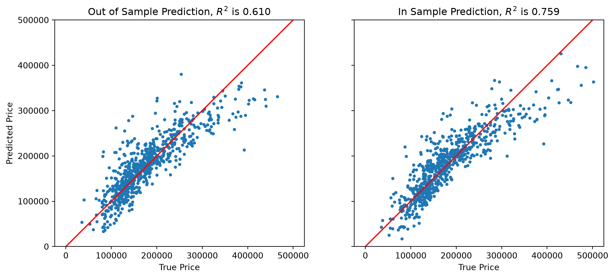
The summary table offers many statistics, but two pictures tell us more: the predictions against the ground truth, and then the residuals against the fitted values.
For each house we compute its predicted sale value according to our model:
\[
\hat{\mathbf{y}} = X\hat{\boldsymbol\beta}
\]
Code
from sklearn.metrics import r2_scorefig, (ax1, ax2) = plt.subplots(1,2,sharey ='row', figsize=(12, 5))y_oos_predict = results.predict(X_test)r2_test = r2_score(y_test, y_oos_predict)ax1.scatter(y_test, y_oos_predict, s =8)ax1.set_xlabel('True Price')ax1.set_ylabel('Predicted Price')ax1.plot([0,500000], [0,500000], 'r-')ax1.axis('equal')ax1.set_ylim([0, 500000])ax1.set_xlim([0, 500000])ax1.set_title(f'Out of Sample Prediction, $R^2$ is {r2_test:0.3f}')#y_is_predict = results.predict(X_train)ax2.scatter(y_train, y_is_predict, s =8)r2_train = r2_score(y_train, y_is_predict)ax2.set_xlabel('True Price')ax2.plot([0,500000],[0,500000],'r-')ax2.axis('equal')ax2.set_ylim([0,500000])ax2.set_xlim([0,500000])ax2.set_title(f'In Sample Prediction, $R^2$ is {r2_train:0.3f}')plt.show()
Ignoring fixed x limits to fulfill fixed data aspect with adjustable data limits.
Ignoring fixed x limits to fulfill fixed data aspect with adjustable data limits.
We see that the model does a reasonable job in the middle of the price range, where most of the houses are.
At both ends the predictions are pulled toward the mean: cheap houses are over-predicted and expensive ones under-predicted. That is not a bug in this particular fit. \(\hat{\mathbf{y}}\) is a projection of \(\mathbf{y}\), so it is the shorter vector and \(\text{Var}(\hat{\mathbf{y}}) \le \text{Var}(\mathbf{y})\): fitted values are always less spread out than the truth. This is Galton’s regression to the mean, now falling out of the algebra.
Note that the \(R^2\) on the (held out) test data is 0.610, against 0.759 in sample. We are not doing as well on test data as on training data (somewhat to be expected).
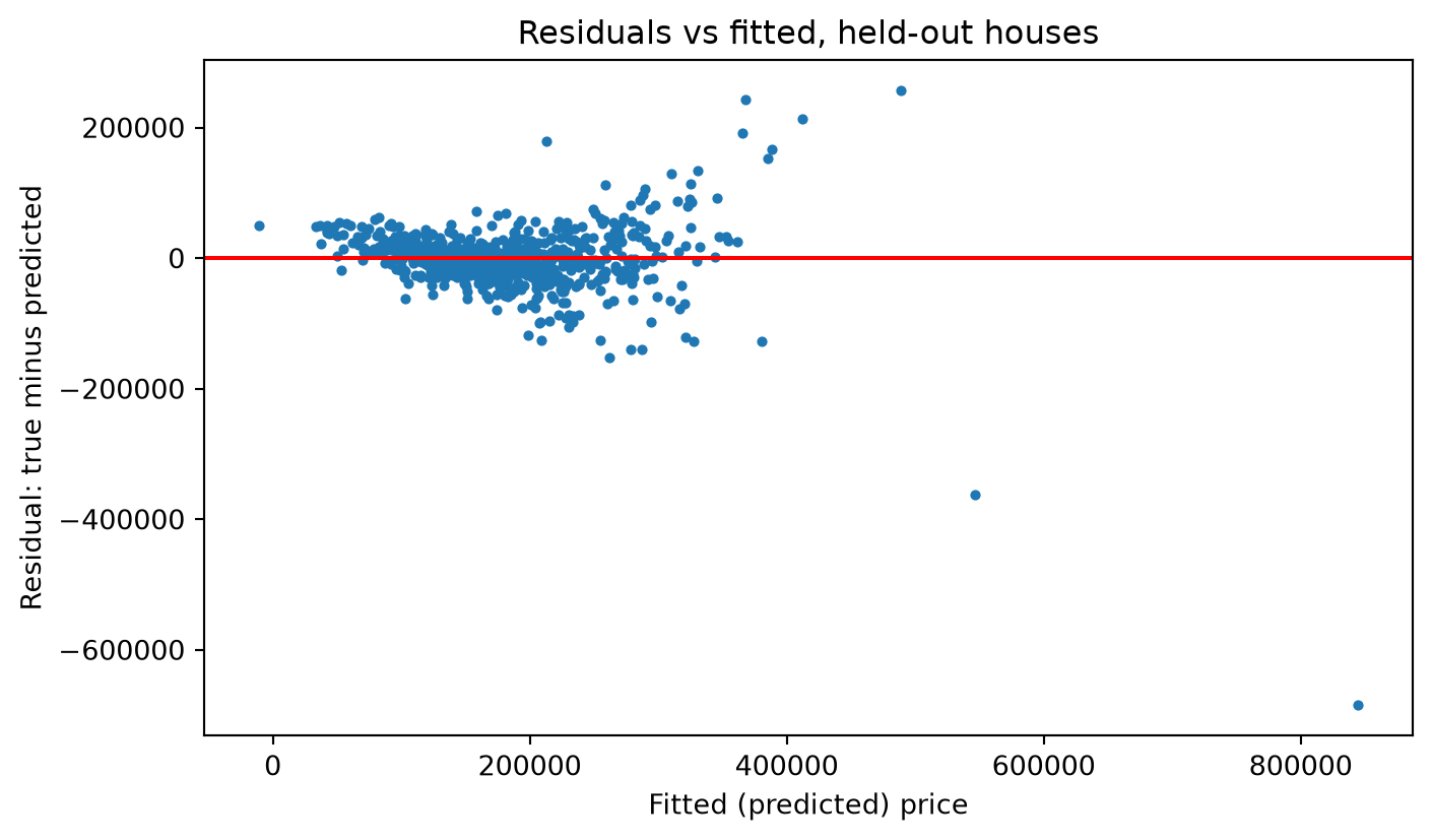
\(R^2\) compresses the fit into one number; the residuals \(\mathbf{e} = \mathbf{y} - \hat{\mathbf{y}}\) show where the model is wrong. Plot them against the fitted values, again for the held-out houses:
A healthy fit shows a flat, even band around zero. This one fans out: the spread of the residuals grows with the predicted price, so the model is far less reliable for expensive houses than for cheap ones (heteroscedasticity). Between roughly $300,000 and $500,000 the residuals are mostly positive – the under-prediction of expensive houses we saw above.
Then there are the two points on the far right: houses the model prices at about $550,000 and $850,000 that sold for hundreds of thousands less. These are the famous Ames outliers – two enormous houses (over 4,000 sq ft of living area) sold under unusual partial sale conditions. Points far out in feature space with huge residuals: a high-leverage problem, and the dataset’s own documentation recommends removing them. The scatter above hid them (they are off its axes); the residual plot does not.
The standard fix for the fan is to model \(\log(\text{SalePrice})\) rather than the price itself: errors become proportional rather than additive, which is more plausible for prices and flattens the fan. The cost is that coefficients then read as percentage changes, not dollars.
Make this plot every time. Three patterns to look for: a bow (a missing nonlinear term), a fan (spread that changes with the fit), and a lone point far out in \(x\) (high leverage, a large \(P_{ii}\)) that can tilt the whole fit. You will practise all three in the activity.
For a better model, we’d also want to consider more features of each house, and perhaps some additional functions such as polynomials as components of our model.
Recap
Linear models are a powerful tool for prediction and inference
Least squares is a projection: the normal equations say the residual is orthogonal to every column of \(X\)
The \(R^2\) statistic provides a simple measure of fit; judge it on held-out data
Coefficients are conditional slopes, each read with the other features held fixed
Plot the residuals against the fitted values: a bow, a fan or a lone high-leverage point says the model is wrong in a way \(R^2\) cannot show
Careful use of the model is required to avoid overfitting