Recap: Natural Language Processing
DS701 Session 21 — Mon Nov 16, 2026


Today’s plan
- 5 min — knowledge-check review
- 20 min — highlights and Q&A (answer or pass — answering always earns credit)
- 50 min — case study: routing a help desk’s tickets
- wrap-up and cold-call check-ins
Knowledge-Check Review
KC 1: The TF-IDF weight
Write down the three pieces of the TF-IDF weight of a term \(t\) in a document \(d\) — term frequency, inverse document frequency, and how they combine — and say in one sentence what kind of term ends up with a large weight. What weight does a term that appears in every document of the corpus get, and why is that the point?
KC 2: Why sparse vectors cannot see synonyms
The lecture notes that with one-hot encodings the similarity of two different words is always 0, while word embeddings put words with similar meanings close together (small angle, high cosine). Explain why the sparse representations — one-hot, bag of words, TF-IDF — can never express that “doctor” and “physician” are related, and what an embedding does differently that makes it possible.
KC 3: Why “bank” gets two vectors
A static embedding (Word2Vec) gives “bank” one vector; a contextual model (BERT) gives “bank” a different vector in “river bank” and in “bank account”. Using the lecture’s description of attention (queries, keys, values, softmax-weighted sum), explain what mechanism lets the second vector depend on the neighbouring words. Then name one task from the lecture where that difference matters and one where a static embedding is good enough.
Highlights
Text → tokens → vectors is the whole game
Models cannot read strings. Every NLP system, from a 1990s search engine to GPT, starts the same way:
- Tokenize — split text into pieces from a finite vocabulary: characters, words, or (transformers) subwords —
token,##ize. Normalize as you go (lowercase, …). - Map tokens to numbers — a token ID is an arbitrary index and carries no meaning.
- Represent — turn IDs into vectors that do encode meaning: sparse (one-hot, bag of words, TF-IDF) or dense (embeddings).
- Everything else — similarity search, clustering, classification, generation — runs on the vectors.
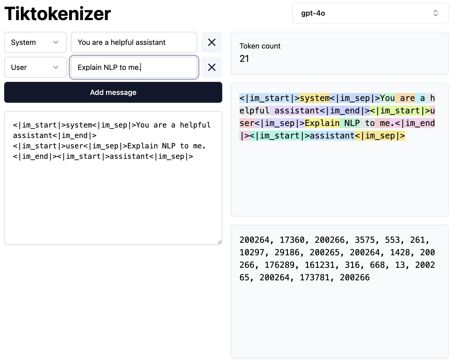
Today’s activity builds steps 1–3 by hand and checks every number against scikit-learn.
Bag of words — and why counts alone mislead
Throw away order and grammar; keep how many times each vocabulary word occurs. A document becomes a vector in \(\mathbb{R}^V\):
| the | cat | sat | on | mat | dog | log | emu | |
|---|---|---|---|---|---|---|---|---|
| “The cat sat on the mat.” | 2 | 1 | 1 | 1 | 1 | 0 | 0 | 0 |
| “The dog sat on the log.” | 2 | 0 | 1 | 1 | 0 | 1 | 1 | 0 |
| “The emu sat on the mat.” | 2 | 0 | 1 | 1 | 1 | 0 | 0 | 1 |
- The largest entry of every row is
the;sat,onare identical across rows. Raw counts mostly say “this is English”. - The words that tell the documents apart (
cat,dog,emu) are the smallest entries — count 1. - Long documents have big vectors, short ones small — length masquerades as content.
- So: down-weight words that are everywhere, and normalize length. That is TF-IDF.
TF-IDF: the formula and what it rewards
\[ \text{tf-idf}(t,d) \;=\; \underbrace{\mathrm{tf}(t,d)}_{\text{frequent here}}\;\times\;\underbrace{\log\frac{N}{\mathrm{df}(t)}}_{\text{rare overall}} \qquad \mathrm{df}(t) = \#\{\text{documents containing } t\} \]
- \(\mathrm{tf}\) rewards a term that is frequent in this document.
- \(\mathrm{idf}\) rewards a term that is rare across the corpus: in every document → \(\log 1 = 0\), gone; in one of \(N\) → \(\log N\), the largest possible.
- On the three sentences (\(N=3\)):
the,sat,onhave \(\mathrm{df}=3 \Rightarrow \mathrm{idf}=0\);cathas \(\mathrm{df}=1 \Rightarrow \mathrm{idf}=\log 3\);mathas \(\mathrm{df}=2 \Rightarrow \log 1.5\). The document vector is now carried bycat,dog,emu,mat,log. - Originally a search-engine ranking function; equally good as the feature matrix for clustering (the newsgroups in Lecture 4) and classification.
TF-IDF in practice: what scikit-learn actually computes
TfidfVectorizer is not the textbook formula. Its defaults:
\[ \mathrm{idf}_{\text{sk}}(t) = \log\frac{1+N}{1+\mathrm{df}(t)} + 1, \qquad\text{then each document row is divided by its } \ell_2 \text{ norm.} \]
- Smoothing (the \(+1\)s): no term is ever weighted exactly 0, no division by zero for a term first seen at query time. Consequence: on a tiny corpus
thecan still top the ranking — the lecture’s table showsthe= 0.617 in sentences 1 and 3 (0.584 in sentence 2), the largest entry of every row. - \(\ell_2\) normalization: documents of different lengths become comparable, and cosine similarity becomes a plain dot product.
- Practical knobs:
stop_words="english",min_df/max_dfto prune the vocabulary,sublinear_tffor \(1+\log\mathrm{tf}\). On thousands of documents the smoothing barely matters; on three it does. - Same object, two names: term–document matrix in IR, feature matrix \(X\) to us — rows are documents, columns are terms, and it is very sparse.
Document similarity via cosine
\[ \cos\theta = \frac{v_1\cdot v_2}{\lVert v_1\rVert\,\lVert v_2\rVert} \]
- Measures direction, not length: a tweet and an essay on the same subject can score high; a document and its double score 1.
- For counts and TF-IDF (non-negative), \(\cos\theta \in [0,1]\); 0 means no shared term at all.
- The lecture’s cat and dog sentences: 0.75 on raw counts (
the,sat,ondo all the work), 0 on textbook TF-IDF, 0.54 with sklearn’s smoothing. - Nearest-neighbour retrieval: the most similar document to a query is \(\arg\max_j \cos(q, d_j)\) — a search engine in one line, and a measurable one: how often is the neighbour on the same subject?
- Same trick makes cosine the distance for \(k\)-means and hierarchical clustering on text (Lecture 4).
The blind spot.
“my laptop will not power on” “notebook fails to boot”
share no term after stop-word removal → cosine exactly 0, however similar the meaning. Sparse lexical vectors see overlap, not synonymy.
Embeddings: from sparse to dense
Sparse (one-hot, BoW, TF-IDF): one axis per word, all axes orthogonal, similarity = literal overlap. Vocabulary-sized and mostly zeros.
Dense embedding: a learned vector of a few hundred dimensions per word; similar meaning ⇒ small angle. Individual coordinates are not interpretable; the geometry is (king − man + woman ≈ queen).
The bridge you already know — LSA. Take the SVD of the TF-IDF matrix (Lecture 12) and keep the top \(k\) directions (Lecture 13): each direction is a combination of terms that co-occur across documents, and projecting a document onto them gives a dense \(k\)-vector. “laptop” and “notebook” load on the same direction, so the two tickets now score \(>0\). Today’s activity stops at the TF-IDF cosine; this is the step after it.
| static (Word2Vec, GloVe) | contextual (BERT, GPT) | |
|---|---|---|
| per word | one vector | one per occurrence |
| “bank” | same vector | river ≠ account |
| how learned | shallow net predicts word ↔︎ context | deep transformer |
| size / cost | 100–300 d, cheap | 768+ d, GPU |
| good for | similarity, clustering | ambiguity, NER, QA, translation |
What attention adds — in one slide
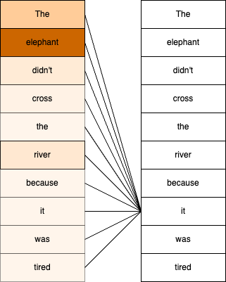
“The elephant didn’t cross the river because it was tired.”
For each token, in parallel over the whole sequence:
- score its query against every token’s key — relevance;
- softmax the scores → weights that sum to 1;
- take the weighted sum of the tokens’ values;
- the token’s representation now carries context — “it” ≈ “elephant”.
\[\text{Attention}(Q,K,V) = \mathrm{softmax}\!\left(\frac{QK^\top}{\sqrt{d_k}}\right)V\]
The weights are computed from the input — that is what makes the embedding contextual, and what neither TF-IDF nor Word2Vec nor LSA can do. Encoder-only (BERT) reads both ways for understanding; decoder-only (GPT) predicts the next token for generation.
The toolkits — pointers, not the point
| Need | Reach for | Where |
|---|---|---|
| tokenize, count, TF-IDF, cosine | sklearn.feature_extraction.text |
today’s activity |
| LSA on top of TF-IDF | TruncatedSVD |
embeddings slide |
| classical text processing, corpora, sentiment lexicons | NLTK | A5 — NLP Packages |
production pipelines: POS, parsing, NER, displacy |
spaCy | A5, lecture NER section |
| topic modeling with transformer embeddings (embed → UMAP → HDBSCAN → c-TF-IDF) | BERTopic | A5, lecture |
| tokenizers and pre-trained transformer models | Hugging Face transformers |
lecture |
| applications on top of LLMs | LangChain | A5 |
Notice how much of the BERTopic pipeline you already own: dimensionality reduction (L13), density clustering (L3–4), TF-IDF per cluster (today). The transformer only supplies step 1.
In-Class Activity
Activity — Case Study 18: Routing and De-duplicating a Help Desk’s Tickets
Goal: a university IT help desk wants new tickets routed to the right team and duplicates of open tickets flagged, and asks what a “word” is to the system and why every ticket seems to match every other. You build the text pipeline by hand — tokenizer, bag-of-words matrix, TF, IDF, TF-IDF — checking each against CountVectorizer / TfidfVectorizer (Parts 1–4), then use cosine similarity to find the nearest open ticket and score it against the team it went to (Part 5). You close with a two-sentence memo: the one preprocessing decision the help desk must sign off on, and the caveat they must hear. The archive cannot be exported yet, so the prototype runs on a hand-made twelve-sentence corpus whose three topics stand in for three teams.
- Work in groups of 2–3. Open your section’s notebook.
- Parts marked (autograded) are submitted to Gradescope; the rest is participation.
- Staff will circulate — be ready to explain any part of your work.
- Dependencies:
numpy,pandas,matplotlib,scikit-learn— no spaCy / NLTK / transformer downloads.


The activity notebook goes live on the day of the lecture. Colab is optional — you can also open it on GitHub and run it locally.
Going deeper
Full lecture notes: Natural Language Processing
- Tokenization and Tokens, Token IDs, and Vocabulary — character, word, subword; the Hugging Face tokenizer demo
- Preprocessing decisions and stemming vs lemmatization
- Sparse Representations — one-hot, bag of words; TF-IDF by hand and as scikit-learn computes it
- Cosine similarity between documents and retrieval
- Word Embeddings, Word2Vec, and Contextual vs Static
- The Attention Mechanism and Queries, Keys, and Values; 3 Types of Transformer Models
- Named Entity Recognition with spaCy; Topic Modeling with BERTopic
- The toolkits, with runnable examples and a Colab notebook: NLP Packages
- The SVD behind LSA: SVD and Low-Rank Approximation and Dimensionality Reduction