Recap: Decision Trees and Random Forests
DS701 Session 9 — Mon Oct 5, 2026


Today’s plan
- 5 min — knowledge-check review
- 20 min — highlights and Q&A (answer or pass — answering always earns credit)
- 10 min — Quiz 1 review (quiz is Wednesday)
- 35 min — case study: prioritizing breast biopsies with trees and forests (small groups)
- wrap-up and cold-call check-ins
Knowledge-Check Review
KC 1: What does a decision tree actually learn?
A tree is fit to a table of loans. What is the learned object, and how is a new loan classified?
Show answer
Answer: the learned object is a set of axis-aligned (e.g. single feature) test conditions (one per internal node) plus a class label at each leaf. A new record is routed down the tree by evaluating one attribute test at a time until it lands in a leaf; the leaf’s majority class is the prediction. No distances, no weights, no gradient — just a nested partition of feature space into boxes.
KC 2: Why not use training error as the splitting criterion?
We split on Home Owner, then Marital Status, then Income, and error dropped to 0%. Why do we bother with Gini or entropy instead of just minimizing error?
Show answer
Answer: classification error counts only the points in each node’s minority class. If a split leaves the same class in the majority in every child, that count doesn’t change, so the error gain is zero, even when the split makes the children much purer.
Home Owner splits the loans (7 No, 3 Yes) into 3 No / 0 Yes and 4 No / 3 Yes:
- Error: 3/10 = 0.3 before, (0 + 3)/10 = 0.3 after. Gain 0, even though one child is now pure.
- Gini: 0.420 before, 0.343 after. Gain 0.077.
The greedy search needs that signal: if error scores many candidate splits as 0 (or as ties), it can’t tell a useful split from a useless one. Gini and entropy are strictly concave, so any split whose children have different class proportions from the parent gets a positive gain.
KC 3: Zero training error — is the tree good?
The full Titanic tree drove training error to ~0 but did worse on the validation set than the one-rule model predict survived = (Sex == female). What happened?
Show answer
Answer: overfitting — the fully grown tree kept splitting until leaves held one or two passengers, so it memorized noise in the training split. It is a low-bias, high-variance model. The one-rule model has high bias but almost no variance, and on this data the variance term dominates the error.
Highlights
1. Growing a tree: greedy recursive partitioning
- Start with all \(N\) records in the root; predict the majority class.
- For every attribute, for every candidate test condition, score the split.
- Take the single best-scoring split, create the children, and recurse independently on each child.
- Stop when a node is pure, or a stopping criterion fires.
The search is greedy and local — the best split now is never revisited, so the tree is not the globally optimal tree. Finding that one is NP-hard.
2. Where can a split go? Depends on the attribute type
- Binary — one obvious split.
- Nominal — multi-way (a branch per value) or binary (a partition of the values into two groups); \(\mathcal{O}(2^k)\) groupings to search.
- Ordinal — binary splits are fine if the ordering is preserved:
{Small, Medium} | {Large, X-Large}is legal,{Small, Large} | {Medium, X-Large}is not. - Continuous — threshold \(x \le \tau\): sort, then sweep the midpoints between consecutive values, \(\mathcal{O}(n)\) after the sort.
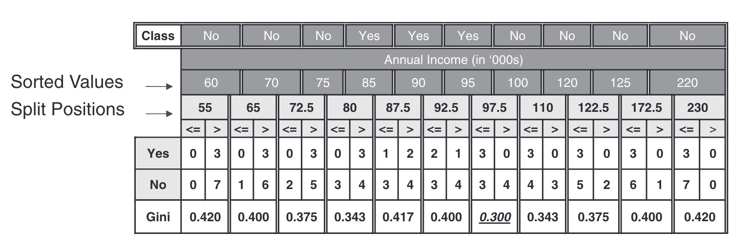
Pick the threshold with the lowest weighted impurity.
3. Impurity measures and how a split is scored
\[ \begin{aligned} \textnormal{Gini} &= 1 - \sum_{i=0}^{c-1} p_i(t)^2 \\ \textnormal{Entropy} &= -\sum_{i=0}^{c-1} p_i(t) \log_2 p_i(t) \\ \textnormal{Error} &= 1 - \max_i p_i(t) \end{aligned} \]
\(p_i(t)\) = relative frequency of class \(i\) at node \(t\); \(0 \log_2 0 = 0\).
Score a split by the weighted average over its children and take the largest gain:
\[ I(\textnormal{ch}) = \sum_{j=1}^{k} \frac{N(v_j)}{N} I(v_j), \quad \Delta = I(\textnormal{parent}) - I(\textnormal{ch}) \]
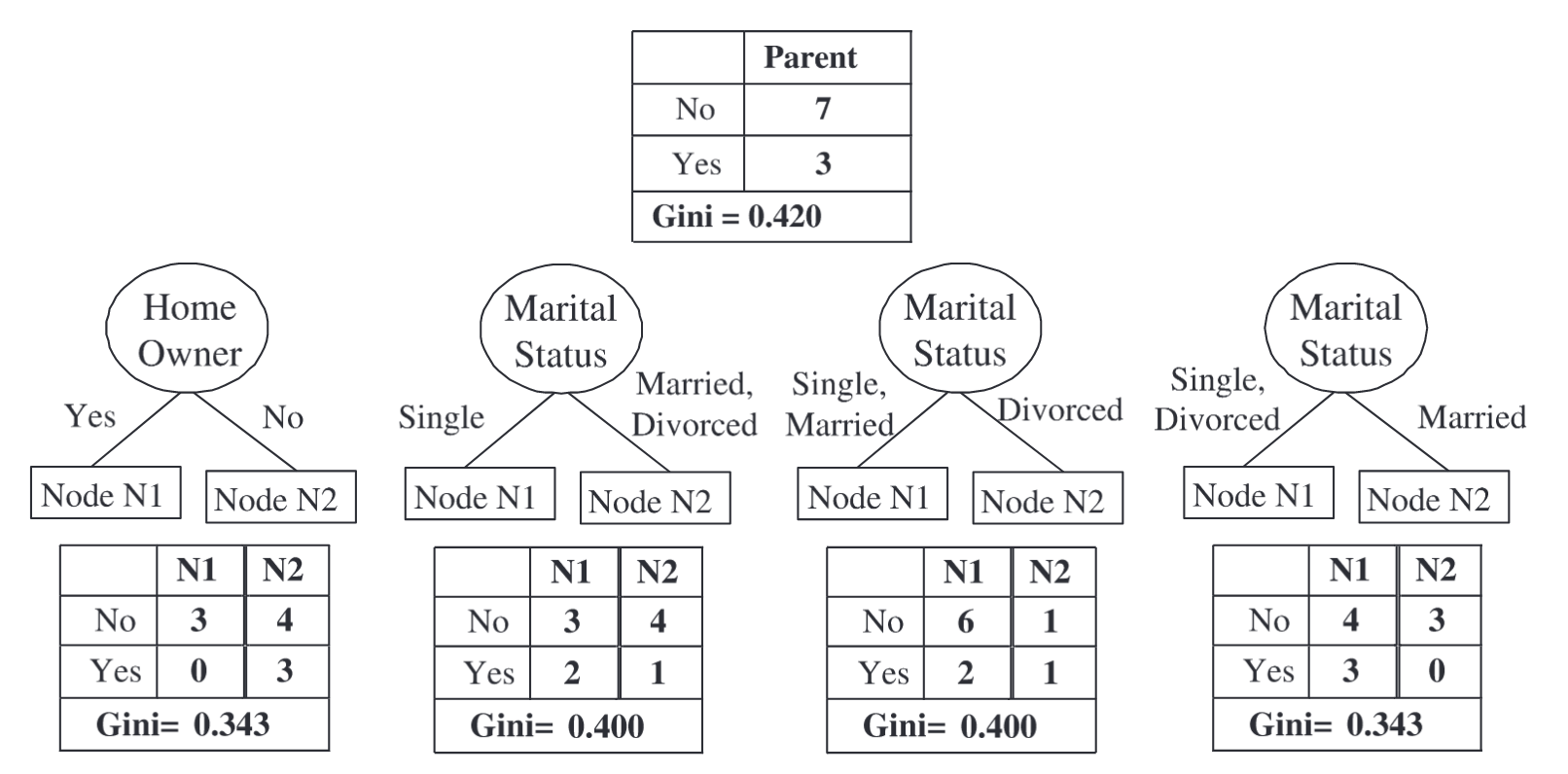
- All three are 0 for a pure node, maximal for a uniform mix.
- Entropy \(\ge\) Gini \(\ge\) Error, always.
- Gini and entropy almost always pick the same split; Gini is cheaper (no logs) and is
scikit-learn’s default. - Largest gain = smallest weighted child impurity, since the parent term is fixed.
4. The pathology: raw gain rewards many-way splits
- Splitting the loans table on the customer ID gives 10 pure leaves and collective entropy exactly 0 — the maximum possible gain — and is completely worthless. It generalizes to nothing.
- Fix 1: binary trees only (CART) — sidesteps varying fan-out entirely.
- Fix 2: gain ratio (C4.5) — divide the gain by the split information \(-\sum_i \frac{N(v_i)}{N}\log_2\frac{N(v_i)}{N}\), penalizing wide splits.
- On the loans data, Marital Status has slightly higher gain (0.195 vs 0.192) but much larger split info (1.486 vs 0.881), so Home Owner wins on gain ratio (0.218 vs 0.131).
- Remember this slide when you read feature importances later.
5. Overfitting: bias, variance, and how to stop it
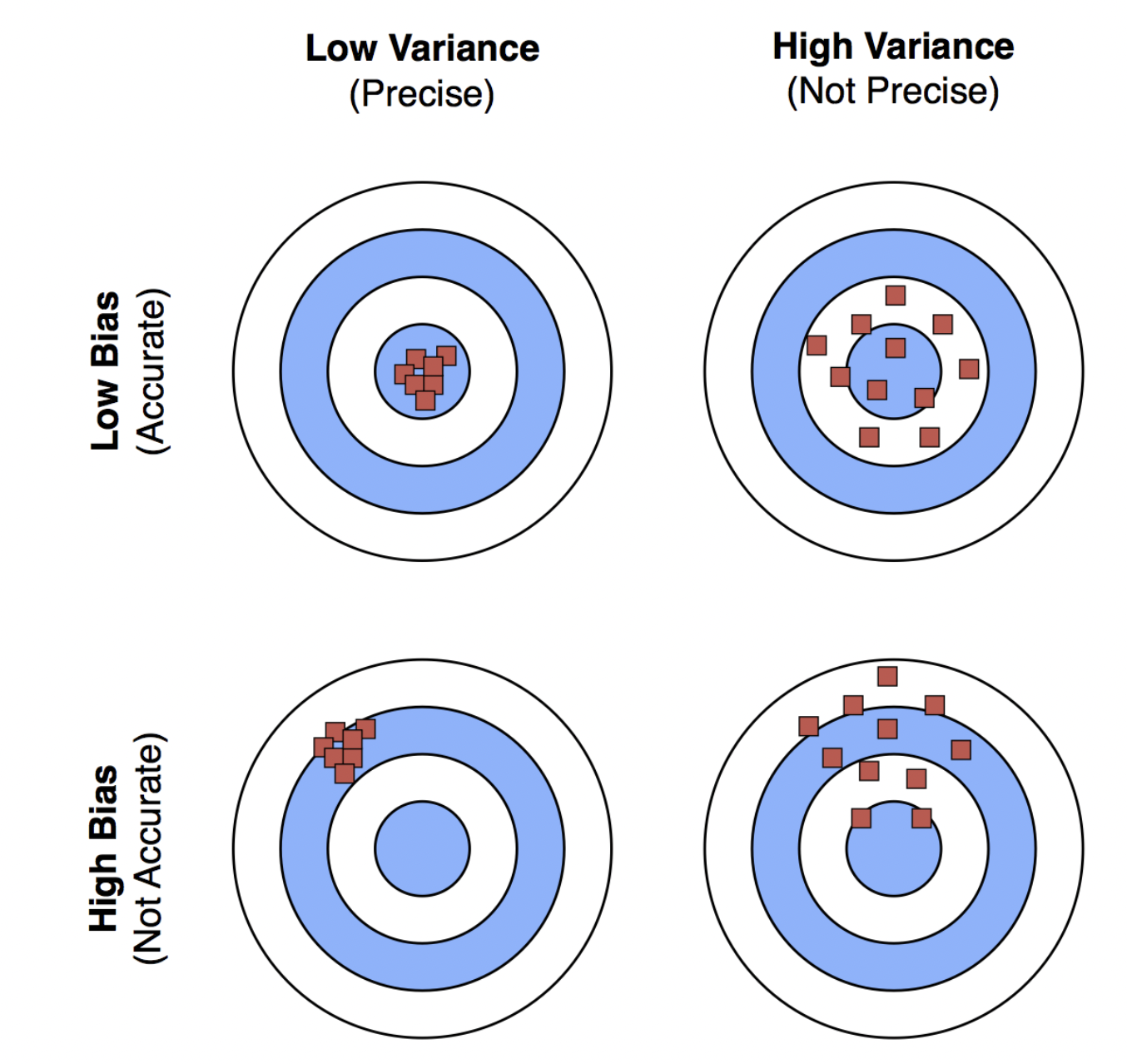
- Bias — error from an over-simple model; a depth-1 stump underfits.
- Variance — error from an over-complex model; a fully grown tree fits the training set exactly and its structure changes wildly under resampling.
- A fully grown tree is the canonical low-bias / high-variance learner — exactly the raw material ensembles want.
- Pre-prune (stopping criteria):
max_depth,min_samples_split/min_samples_leaf, minimum impurity decrease. - Post-prune: grow fully, then collapse subtrees that don’t pay for themselves on held-out data (
ccp_alpha). - On Titanic, both
min_samples_split=20andmax_depth=3beat the unrestricted tree on validation error — less tree, better model.
6. Bagging: average away the variance
- Draw \(B\) bootstrap samples (sample \(N\) records with replacement).
- Fit a fully grown, unpruned tree on each — keep bias low on purpose.
- Predict by majority vote across the \(B\) trees.
- Averaging \(B\) noisy, roughly independent predictors cuts the variance term without inflating bias.
- Free bonus: each tree omits ~37% of the data, so the out-of-bag records give a validation estimate with no separate split.
Catch: bagged trees are correlated. If one feature dominates, every tree splits on it first and the trees look nearly identical — so averaging buys much less than it should.
7. Random forests = bagging + feature subsampling
- Everything bagging does, plus: at each node, consider only a random subset of \(m\) features (
max_features, commonly \(m \approx \sqrt{p}\)). - This forces different trees to use different features, decorrelating them, which is what makes the average actually pay off.
- Each base tree gets slightly worse; the ensemble gets substantially better.
- The lecture’s forest never names this knob — in today’s activity you sweep
max_featuresfrom 1 to all 30 and measure the trees decorrelating (their pairwise prediction correlation drops) while the OOB score barely moves. - Almost no tuning needed: more trees never hurts accuracy, it just costs time.
On Titanic, a 100-tree RandomForestClassifier beat every single tree we fit. A forest is a strong, low-effort baseline for tabular data — no feature scaling, mixed types welcome, automatic feature selection. Try one before anything fancier.
8. Feature importance — read it with suspicion
Trees hand you an importance score for free. Four ways it will mislead you:
- Cardinality bias — impurity-based importance inflates high-cardinality and continuous features (the customer-ID effect, again).
- Correlated features split the credit — two near-duplicate strong features each look half as important as either would alone.
- Computed on training data — a feature can score high purely by memorizing noise. Prefer permutation importance on a held-out set.
- It is not causal, and it is not signed — importance says a feature was used, not which direction it pushes or why.
In-Class Activity
Case study: prioritizing breast biopsies with trees and forests
Goal: advise a consortium of Boston hospitals on whether nucleus measurements from breast biopsies can flag likely-malignant samples — find the best single cutoff, choose a tree depth that generalizes, and decide whether a random forest is worth giving up a readable tree.
- Work in groups of 2–3. Open the notebook for your section — the data split differs, so the other section’s numbers are wrong for you.
- Parts 1–3 are autograded and submitted to Gradescope.
- Finish with the report out: what you would tell the clinical team, and one takeaway to pair-share with a neighboring team.
- Staff will circulate — be ready to explain any part of your work.


The activity notebook goes live on the day of the lecture. Colab is optional — you can also open it on GitHub and run it locally.
Going deeper
Full lecture notes: Decision Trees and Random Forests
- Specifying the Test Condition — attribute types and split shapes
- Impurity Measures and the worked Impurity Examples
- Collective Impurity of Child Nodes — the weighted-average score
- Gain Ratio and the comparison table
- Splitting Continuous Attributes
- Bias and Variance, Stopping Criteria, Random Forests
Reference: Tan, Steinbach, Karpatne & Kumar, Introduction to Data Mining, Ch. 3–4.