Recap: \(k\)-Means Clustering
DS701 Session 4 — Wed Sep 16, 2026


Today’s plan
- 5 min — knowledge-check review
- 20 min — highlights and Q&A (answer or pass — answering always earns credit)
- 60 min — in-class activity (small groups)
- wrap-up and cold-call check-ins
Knowledge-Check Review
KC 1: What does \(k\)-means minimize?
Name the quantity and write it as a formula.
Show answer
Answer: the Within-Cluster Sum of Squares (WCSS), a.k.a. the inertia:
\[ \underset{C_1, \dots, C_K}{\arg\min} \hspace{1em} \sum_{k=1}^K \hspace{1em} \sum_{x\in C_k} \Vert x-c_k\Vert^2. \]
For every point, the squared Euclidean distance to its own cluster center, summed over all points. In scikit-learn this is kmeans.inertia_.
KC 2: One iteration by hand
Points \(1.2,\ 1.8,\ 2.1,\ 7.3,\ 7.9,\ 8.2,\ 9.1,\ 10.5\), initial centers \(A = 4.0\), \(B = 11.0\).
Show answer
Assign — closest center wins (watch \(7.9\): \(|7.9-4.0| = 3.9\) vs. \(|7.9-11.0| = 3.1 \Rightarrow B\)):
| Cluster | Points |
|---|---|
| A | 1.2, 1.8, 2.1, 7.3 |
| B | 7.9, 8.2, 9.1, 10.5 |
Update — center of mass of each cluster:
\[ A' = \frac{1.2+1.8+2.1+7.3}{4} = 3.1, \qquad B' = \frac{7.9+8.2+9.1+10.5}{4} = 8.9 \]
Next round, \(7.3\) defects to \(B\) (\(4.2\) vs. \(1.6\)) and we settle at \(A^\ast = 1.7\), \(B^\ast = 8.6\).
KC 3: Why scale the features?
Cluster customers on age (18–80) and income ($20k–$200k), unscaled. What determines the clusters?
Show answer
Answer: income, and only income.
- Assignment uses Euclidean distance, and squared income differences are ~\(10^6\) times larger than squared age differences.
- A one-dollar difference in income counts about as much as a whole category of a binary feature.
- Fix: center each feature at zero and rescale to unit standard deviation, so every feature gets a comparable say in the distance.
Highlights
What are we actually asking for?
A clustering is a grouping of data objects such that objects within a group are similar and objects in different groups are dissimilar.
So we want to:
- minimize intra-cluster distances
- maximize inter-cluster distances
And it is unsupervised — no labels go in, and any labels we put on the clusters we invent afterwards.
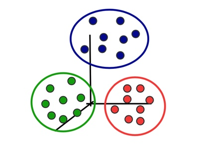
Partitional setup for \(k\)-means: data are points in \(\mathbb{R}^d\), every object belongs to one and only one cluster (mutually exclusive), the clusters cover everything (exhaustive), and \(K\) is given in advance.
Hard problem, easy algorithm
- Minimizing WCSS exactly is NP-hard for \(d \ge 2\) — no efficient exact algorithm is expected.
- \(k=1\) and \(k=n\) are the easy corner cases (global mean; every point its own center, WCSS \(=0\)).
- Nonetheless: Lloyd’s algorithm (1957) is a simple heuristic that works very well in practice.
- Voted a top-10 data mining algorithm, and independently rediscovered several times.
- Careful with the wording: the \(k\)-means problem \(\neq\) the \(k\)-means algorithm.
Lloyd’s algorithm
- Pick \(K\) cluster centers \(\{c_1, \dots, c_K\}\)
- random data points, or \(k\)-means++
- Assign: define \(C_j\) as the points closest to center \(c_j\)
- Update: set \(c_j\) to the center of mass of \(C_j\)
- Repeat step 2 until convergence
- centers move below a threshold, or inertia changes below a threshold, or max iterations
Neither step 2 nor step 3 can increase WCSS \(\Rightarrow\) it always converges — but only to a local minimum.
Initialization matters
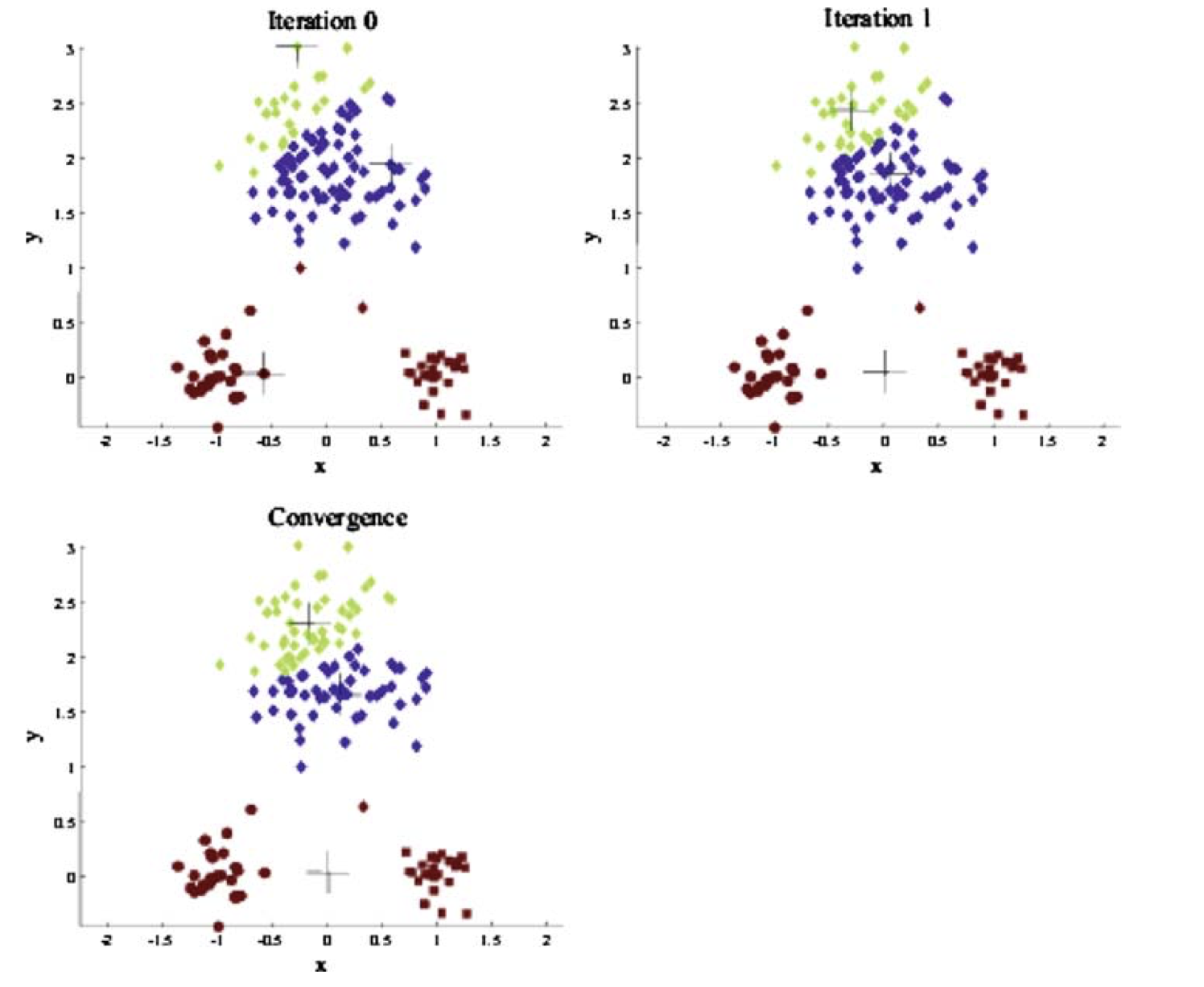
- Same data, same \(K\), different random start \(\Rightarrow\) different answer.
- A bad start gets stuck: the algorithm can never climb back out, because it never increases WCSS.
- Strategy: pick initial centers that are far apart — this is \(k\)-means++.
- It is
scikit-learn’s default, andn_initrestarts the whole thing several times and keeps the best WCSS.
Choosing \(K\)
\(K\) is our first hyperparameter: a parameter that must be set before the model parameters (the centers) can be learned.
WCSS alone can’t pick it — WCSS decreases monotonically in \(K\), all the way to \(0\) at \(K = n\).
So: sweep \(K = 1, 2, 3, \dots\), fit each, and score it.
- Elbow method — plot WCSS vs. \(K\) and look for the bend where the marginal gain flattens.
We’ll also talk about the silhouette coefficient in an upcoming lecture.
Where \(k\)-means breaks
Assignment is “nearest center”, so cluster regions are straight-sided Voronoi cells and clusters are implicitly assumed to be spheres around their center.
- Non-spherical — two half-moons get sliced by a straight boundary.
- Anisotropic — stretched/rotated blobs, same failure after a linear transformation.
- Unequal variance — squared distances make the wide cluster expensive, so it gets split.
- Unequal sizes — the objective prefers roughly balanced, equal-radius cells (500/100/10 will not survive).
- Bad init — a local minimum of WCSS.
- Wrong \(K\) — ask for 2 and you get 2, whatever the data says.
Feature scaling
Because \(k\)-means looks for spherical clusters in Euclidean distance, the units of each feature are part of the model.
\[ \begin{bmatrix}\text{age } 27\\\text{income } 75000\\\text{gender } 0\end{bmatrix}, \qquad \begin{bmatrix}\text{age } 45\\\text{income } 42000\\\text{gender } 1\end{bmatrix} \]
Standard remedy, per feature and independently:
- subtract the mean (centers the feature at zero), then
- divide by the standard deviation (puts every feature on a comparable range).
Whenever you build or pick a distance metric, think about feature scale first.
Where it works well
\(k\)-means is a workhorse when the assumptions roughly hold:
- Customer segmentation — spending / order value / order count \(\rightarrow\) personas (scale first: dollars vs. counts).
- Iris — recovers the three species almost exactly; setosa is cleanly separated, versicolor/virginica overlap a little.
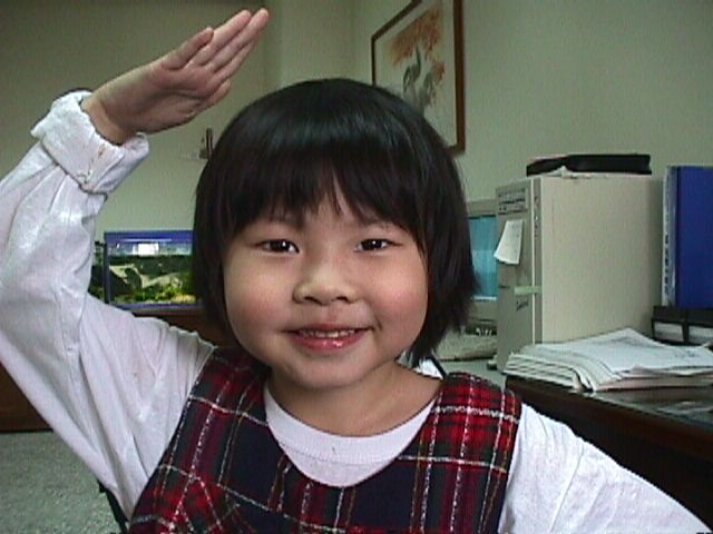
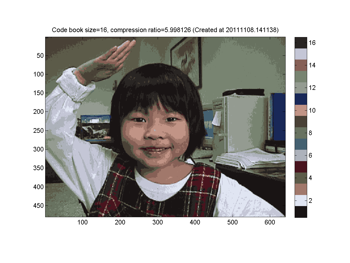
- Image compression — cluster pixels in \((R,G,B)\) space, replace each pixel with its centroid. \(k=16\) means a 4-bit palette index instead of 24 bits: \(24/4 = 6\times\).
In-Class Activity
Activity: \(k\)-Means from scratch and in scikit-learn
Goal: implement one Lloyd’s iteration yourself, check it against sklearn.cluster.KMeans, then the stretch — sweep \(k\), and settle a case where the elbow is not clear — and finally break \(k\)-means on purpose and diagnose why.
- Work in groups of 2–3.
- Parts marked (autograded) are submitted to Gradescope; the rest is participation.
- Staff will circulate — be ready to explain any part of your work.
- Dependencies:
numpy,matplotlib,scikit-learnonly.


The activity notebook goes live on the day of the lecture. Colab is optional — you can also open it on GitHub and run it locally.
Going deeper
Full lecture notes: \(k\)-Means Clustering
- Minimizing a Cost Function — the WCSS objective
- The \(k\)-means Algorithm — the four steps, worked on well-separated and overlapping blobs
- Limitations of \(k\)-means — non-spherical, anisotropic, unequal size and variance
- Choosing a Good Initialization — \(k\)-means++
- Choosing the right \(k\) — hyperparameters
- Feature Scaling
Also see:
Other clustering evaluation metrics:
- Rand Index – when you have ground truth labels
- Silhouette Coefficient – when you don’t
Also see k-means++ initialization
Next up: hierarchical clustering (04) — clusters without choosing \(k\) up front.