Recap: Dimensionality Reduction — PCA and t-SNE
DS701 Session 16 — Wed Oct 28, 2026


Today’s plan
- 5 min — knowledge-check review
- 20 min — highlights and Q&A (answer or pass — answering always earns credit)
- 35 min — case study: can thirteen lab measurements tell wines apart
- wrap-up and cold-call check-ins
Knowledge-Check Review
KC 1: The first step, and why
What is the very first step of PCA, and in one sentence, why is it required?
KC 2: PCA and the SVD
If the centered data matrix has SVD \(X = U\Sigma V^T\), where do the principal components live, and how do the singular values relate to the eigenvalues of the covariance matrix \(S\)?
KC 3: Two things a t-SNE plot does not tell you
Name two things you should not conclude from a t-SNE plot, and one thing t-SNE genuinely does preserve.
Highlights
1. PCA in one picture
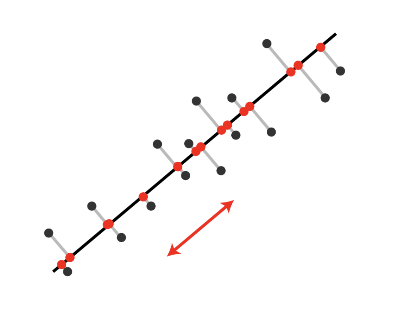
The sum of variances of the projected points is a maximum.
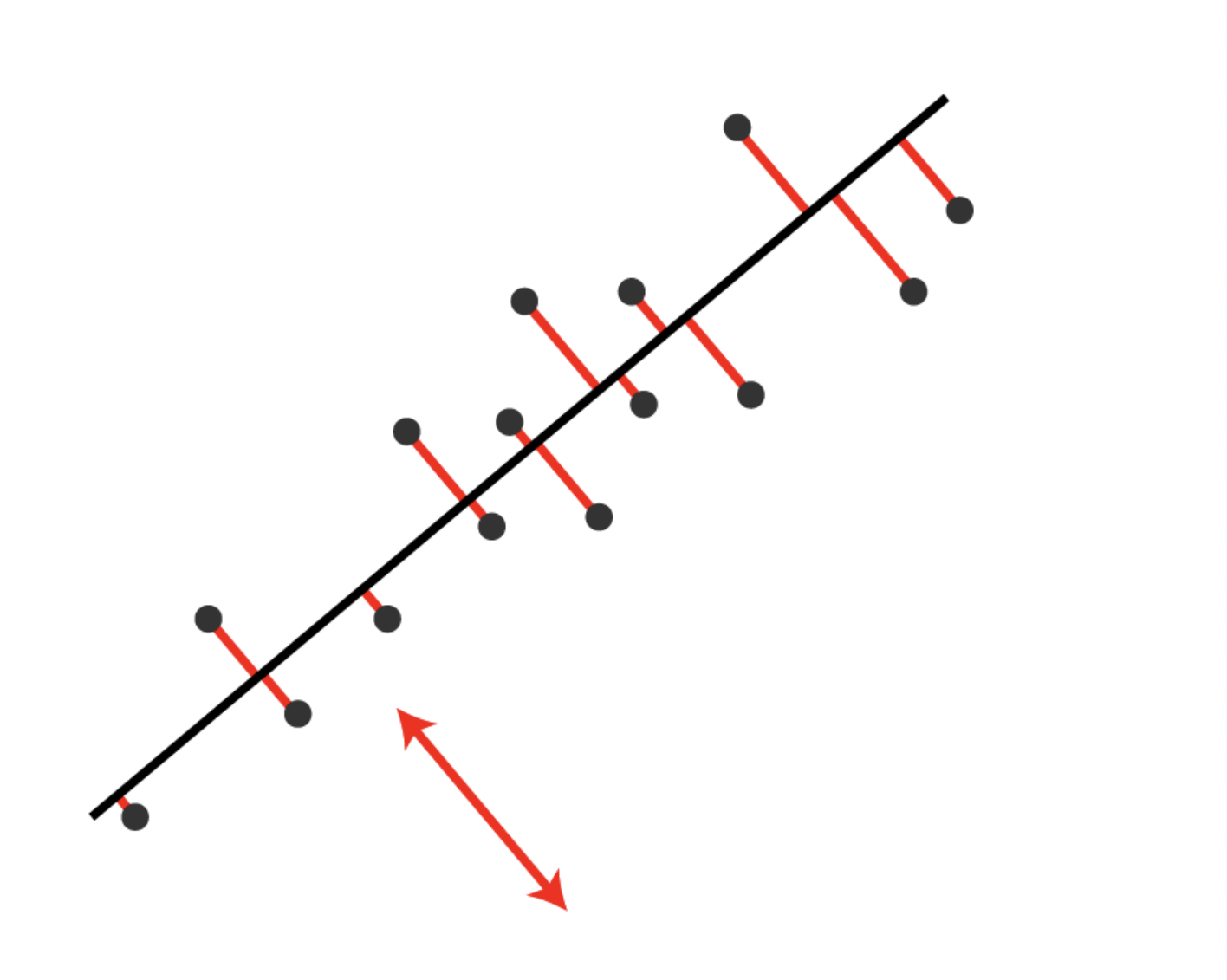
The sum of residuals (squared distances from points to the line) is a minimum.
These are the same optimization: for centered data, projected² + residual² is a fixed total, so maximizing one minimizes the other.
2. The PCA recipe
- Center: subtract column means, \(X_0 \rightarrow X\).
- Covariance: \(S = \frac{1}{m-1}X^{T}X\) — symmetric, \(n \times n\), one row/column per feature.
- Spectral decomposition: \(S = V\Lambda V^{T}\) with \(\lambda_1 \ge \lambda_2 \ge \dots \ge \lambda_n\) and orthonormal \(V\).
- Truncate: keep the first \(d\) columns of \(V\) as \(V'\).
- Project: \(Y = XV' \in \mathbb{R}^{m \times d}\).
Step 3 is legal because \(S\) is real symmetric — that is what guarantees real eigenvalues and perpendicular principal directions.
3. What \(Y = XV'\) actually does
Rotation, then projection.
- \(V'\) defines \(d\) new orthogonal axes pointing along the directions of maximum variance.
- Each point becomes its coordinates along those axes: \[\mathbf{y}_i = \begin{bmatrix} \mathbf{x}_i \cdot \mathbf{v}_1 & \mathbf{x}_i \cdot \mathbf{v}_2 & \cdots & \mathbf{x}_i \cdot \mathbf{v}_d\end{bmatrix}\]
- The discarded directions are the low-variance ones.
Intuition: find the “best viewing angle.” Data that is a pancake in 3D really lives in a 2D plane — \(V'\) orients that plane, \(Y\) gives coordinates inside it.
4. In practice: PCA is the SVD of the centered data
\[X = U\Sigma V^{T} \quad\Longrightarrow\quad X^{T}X = V\Sigma^{2}V^{T}\]
- Principal components = right singular vectors \(V\).
- Eigenvalues of \(S\) = \(\sigma_i^{2}/(m-1)\).
- Projected data \(Y = XV' = U'\Sigma'\).
- Last lecture’s rank-\(d\) truncated SVD is PCA with \(d\) components — once the data is centered.
Nobody forms \(S\) and eigendecomposes it. Reasons: numerical stability (squaring \(X\) squares the condition number), efficiency (truncated SVD gets just the top \(d\)), and it hands you \(V\) directly.
5. Choosing \(d\): explained variance and the scree plot
Total variance \(T = \lambda_1 + \lambda_2 + \dots + \lambda_n\).
- Explained variance of component \(i\): \(\;\lambda_i / T\).
- Cumulative explained variance through \(k\): \(\;\sum_{i=1}^{k}\lambda_i/T\), reaching 1 at \(k = n\).
- Scree plot: \(\lambda_i/T\) vs. \(i\). Look for the elbow — where the curve flattens into noise.
- Threshold rule: smallest \(k\) with cumulative \(\ge 0.90\) (or 0.95).
Caution: variance \(\ne\) usefulness. A low-variance direction can still be the one that separates your classes.
6. To scale or not to scale
Same four people, height in feet vs. centimeters:
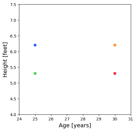
Height in feet — variance runs horizontally (age).
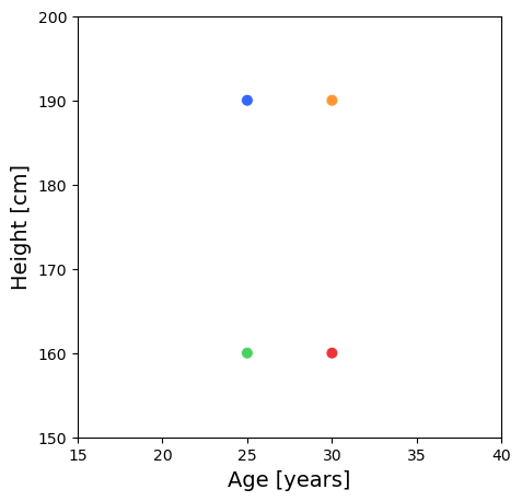
Height in cm — variance now runs vertically.
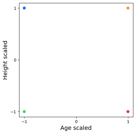
Standardized — variance shared evenly.
Variance is unit-dependent, so PCA is not scale-invariant. Standardizing means you are doing PCA on the correlation matrix — best practice whenever features have different units or scales.
7. Why this matters: genes mirror geography
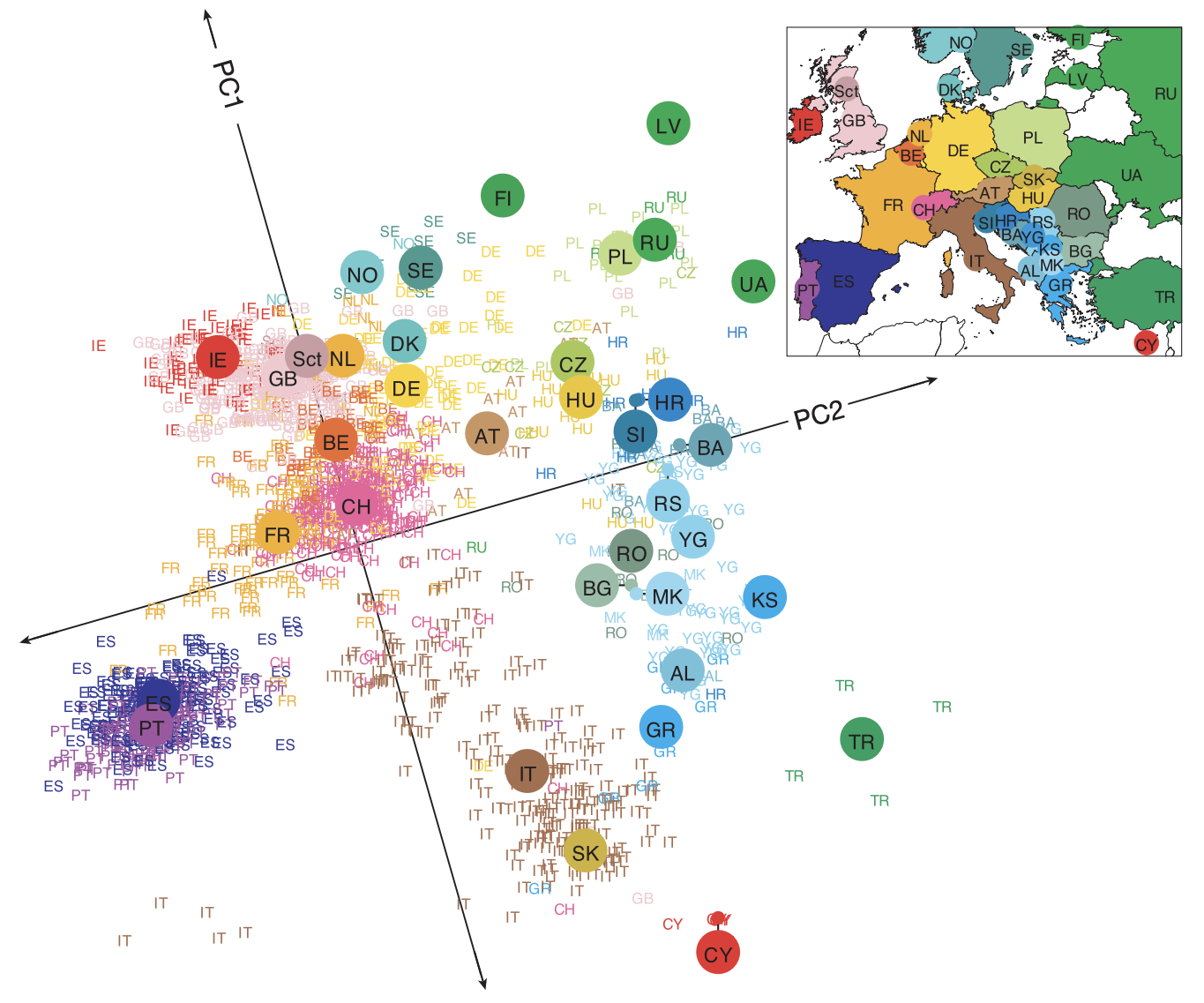
- ~3000 individuals × ~500k SNPs (each entry a 0/1/2 minor-allele count), reduced to two components; the 1387 people with all four grandparents from one country are plotted.
- PC1 and PC2 essentially reconstruct the map of Europe — latitude and longitude fall out of the DNA.
- Two numbers can locate a person’s birthplace to within a few hundred kilometers.
8. t-SNE: a different objective entirely
- High-D similarity: Gaussian around each point, \(p_{j\vert i} \propto \exp(-\|x_i - x_j\|^{2}/2\sigma_i^{2})\), symmetrized into \(p_{ij}\). The bandwidth \(\sigma_i\) is set per point by the perplexity (effective number of neighbors; typical 5–50, default 30).
- Low-D similarity: Student-t, \(q_{ij} \propto (1 + \|y_i - y_j\|^{2})^{-1}\).
- Fit: gradient descent on \(KL(P\|Q) = \sum_{i \ne j} p_{ij}\log\frac{p_{ij}}{q_{ij}}\), moving the \(y_i\) until the low-D neighborhoods match the high-D ones.
The asymmetry is the point: heavy t-distribution tails let a moderate 2D distance stand in for a large high-D distance, relieving the crowding problem.
9. PCA vs. t-SNE
| Feature | PCA | t-SNE |
|---|---|---|
| Speed | Fast | Slow (>10k points hurts) |
| Purpose | Dimensionality reduction | Visualization |
| Preserves | Global variance | Local neighborhoods |
| Linear? | Yes | No |
| Deterministic? | Yes | No (random init) |
| Distances | Meaningful | Not meaningful |
| Reusable transform? | Yes | No |
Best practice: PCA down to ~50 dimensions first, then t-SNE.
10. t-SNE cautions — read this before you interpret a plot
Don’t trust
- cluster sizes (dense regions get inflated)
- distances between clusters
- any structure that isn’t stable across seeds
- the coordinates as model features
Do
- standardize / PCA-preprocess first
- try 3–5 perplexities (5, 15, 30, 50)
- rerun with different seeds
- read only local neighborhoods
“Cluster A is bigger than B and far from C, so A and B are related” — every part of that sentence is unsupported.
In-Class Activity
Activity — Case Study 13: Can Thirteen Lab Measurements Tell Wines Apart?
Goal: advise an analytical-chemistry lab that runs a 13-assay panel on every wine lot and has been handed a vendor’s t-SNE plot “proving” the panel separates wines by producer — standardize and run PCA to find how many of the 13 measurements carry the signal, measure what keeping \(d\) of them loses and verify it against the SVD, then write the lab a two-sentence memo and a rule for what the vendor’s plot can and cannot claim.
- Work in groups of 2–3.
- Parts 1–2 are autograded and submitted to Gradescope; the discussion and the memo are participation.
- Finish with the report out: the recommendation and the one caveat for the lab, plus your rule for reading a t-SNE plot — staff will circulate and ask, so agree on your answer.


The activity notebook goes live on the day of the lecture. Colab is optional — you can also open it on GitHub and run it locally.
Going deeper
Full lecture notes: Dimensionality Reduction — PCA + t-SNE
Prerequisite refresher: Eigendecomposition