Recap: Generalization — Why Training Error Lies
DS701 Session 8 — Wed Sep 30, 2026


Today’s plan
- 5 min — knowledge-check review
- 20 min — highlights and Q&A (answer or pass — answering always earns credit)
- 60 min — in-class activity (small groups)
- wrap-up and cold-call check-ins
Knowledge-Check Review
KC 1: The contract
State the “supervised contract” — the assumption the lecture says makes it possible for a rule learned on training data to say anything about data it has never seen — and give one concrete situation in which the contract is broken.
Show answer
Answer. Training pairs \((\mathbf{x}_i, y_i)\) and future pairs \((\mathbf{x}_j, y_j)\) are drawn independently from the same distribution (i.i.d.) — the rule linking \(\mathbf{x}\) to \(y\) is the same for the data you learn from and the data you will predict on. The future looks like the past.
Broken whenever the distribution shifts: a new sensor or protocol, a new year or season, a new population or region, a policy change that alters behaviour, a training set selected in a way the future will not be. Then no held-out score means anything — every claim about generalization is conditional on the contract.
KC 2: Why training error only goes down
In the polynomial curve-fitting example, the training error reaches zero at \(k = 9\) while the test error is smallest at \(k = 3\). Explain why training error can only go down (never up) as \(k\) increases, and why that makes it useless for choosing \(k\). Then say which of bias and variance the \(k = 9\) model suffers from, and which the \(k = 1\) model — in one sentence each.
Show answer
Monotone: a degree-\(k\) polynomial is a special case of degree \(k+1\) (top coefficient \(= 0\)), so the least-squares optimum over the bigger family is never worse on the training points. With 10 points and 10 coefficients (\(k = 9\)) it interpolates the noise and hits zero.
Useless for choosing \(k\): it always prefers the most complex model — it selects the fit to the noise, i.e. it overfits.
\(k = 9\) — variance: refit on another 10 noisy points and you get a completely different wiggle. \(k = 1\) — bias: a line cannot follow a sine no matter how much data it sees; it underfits.
KC 3: Choosing a depth with 5-fold CV
You have 200 labelled rows and must choose the maximum depth of a decision tree (a hyperparameter). Describe how you would use 5-fold cross-validation to choose it, and say what role — if any — the test set plays in that choice. Why is 5-fold CV preferable to a single random train/validation split when the data is this small?
Show answer
Protocol. Lock away a test set (say 40 rows). Partition the other 160 once into 5 folds of 32. For each candidate depth: train on 4 folds, score the 5th, rotate so every fold is validation exactly once, average the 5 errors. Pick the depth with the lowest CV error, refit on all 160, and only then score the test set — once.
The test set has no vote. The moment it influences a choice it stops being an unbiased estimate of future error.
Why \(K\)-fold and not one split: with few rows a single validation set is small and its error is noisy — one unlucky partition can flip the choice. \(K\)-fold tests every row once and trains on it \(K-1\) times, averaging the partition away and wasting nothing.
Highlights
Everything supervised rests on one contract
Given training pairs \(\{(\mathbf{x}_i, y_i)\}_{i=1}^N\), learn a rule that predicts \(y_j\) for an \(\mathbf{x}_j\) not in the training data.
Two assumptions make that tractable:
- There is a family of functions to search through (large!).
- The contract: \((\mathbf{x}_i, y_i)\) and \((\mathbf{x}_j, y_j)\) are drawn i.i.d. from the same distribution — the rule for the training data is the rule for the future.
Two consequences we will lean on all term:
- the future must look like the past — a new sensor, year, or population voids every score you computed;
- the test data must stay untouched — it is our stand-in for the future, and it can only play that role if it never influenced a decision.
Training error lies
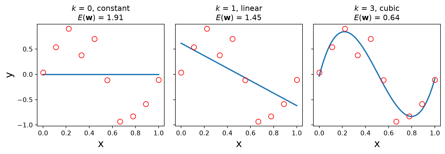
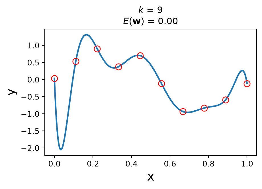
\(N = 10\) points, \(y = \sin(2\pi x) + \varepsilon\). Least squares finds the \(\mathbf{w}^*\) that minimises training error \(E(\mathbf{w}) = \sum_n [f(x_n, \mathbf{w}) - y_n]^2\). Training error: \(1.91 \to 1.45 \to 0.64 \to\) 0.00 at \(k = 9\) (10 coefficients, 10 points — it interpolates). Which one would you bet on for the next point?
The money plot: train vs test
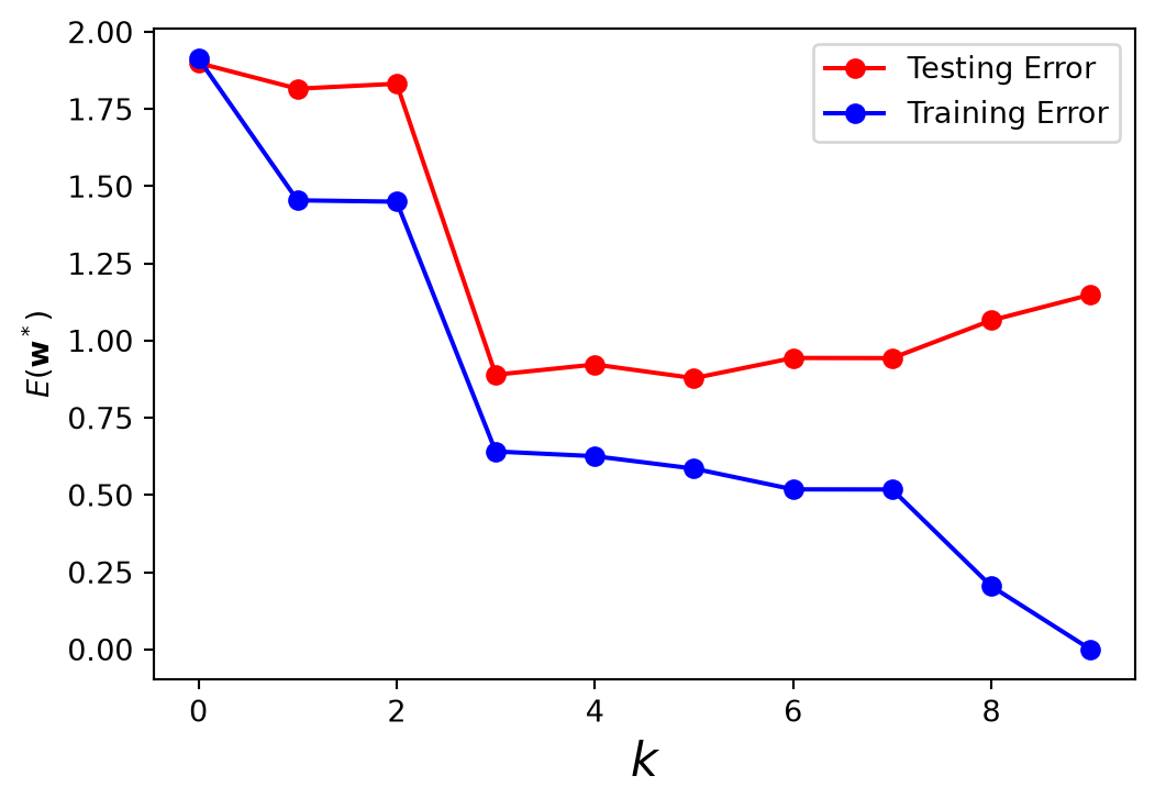
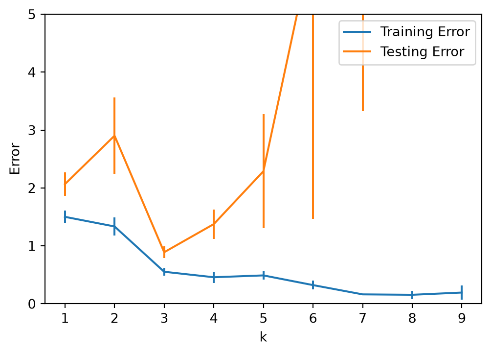
- Score every fit on fresh points from the same generator.
- Training error falls monotonically — a bigger family can always reproduce a smaller one — and reaches zero.
- Test error falls, bottoms out at \(k = 3\), then rises.
- Training ↓ while test ↑ is overfitting: fitting the training data “too well” — noise included.
Why it happens: too many parameters for the data; a model more complex than the phenomenon. What helps: more data, less complexity (hyperparameters), regularization.
Two ways to be wrong
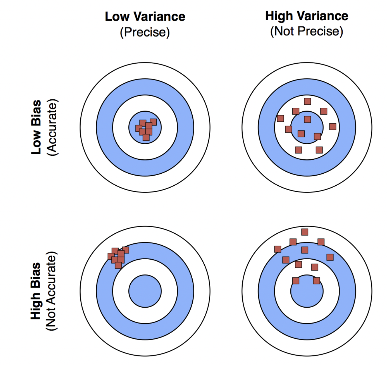
Bias — the model is too simple to capture the pattern; it underfits (\(k = 0, 1\)). Refit it on new data and it is wrong the same way every time.
Variance — the model is so flexible it fits the noise; it overfits (\(k = 9\)). Refit it on a different sample from the same distribution and you get a very different answer.
Both are defined over repeated draws of the training set — which is exactly what you will do in Part 3 today.
The trade-off is the U-shape
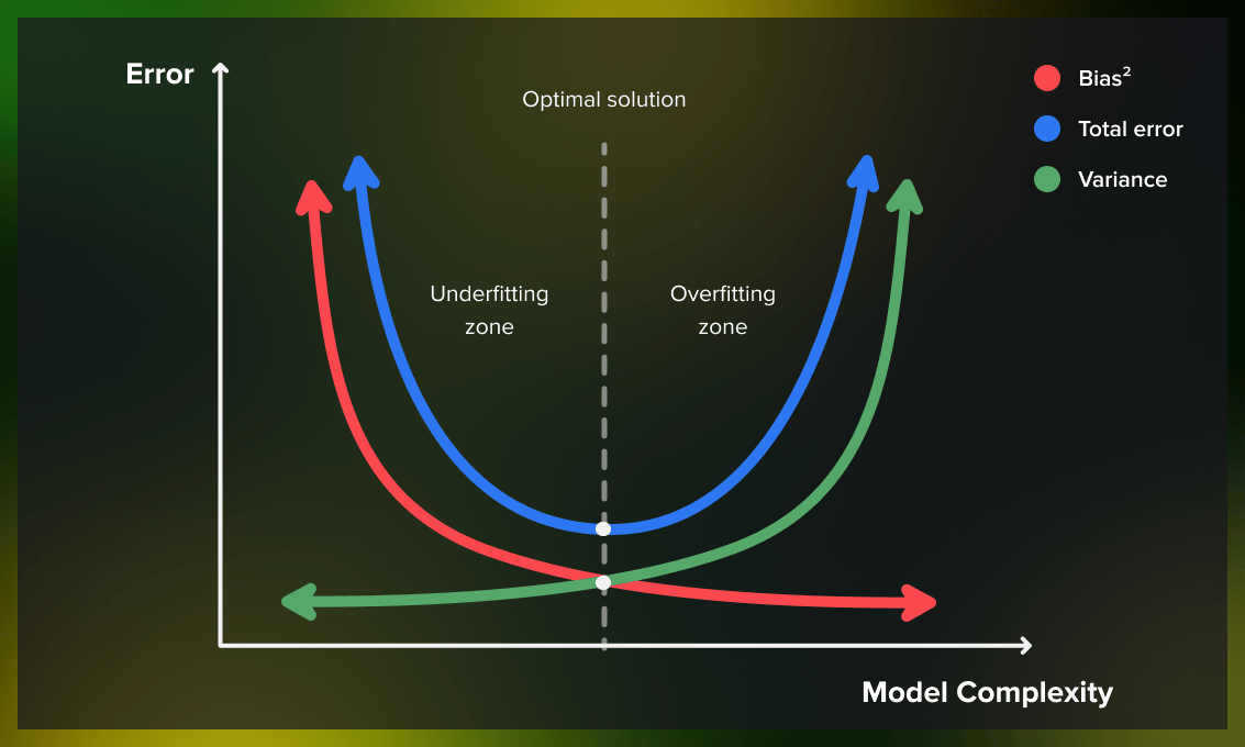
- More flexibility: bias ↓, variance ↑.
- Left of the minimum, bias dominates; right of it, variance.
- The test-error minimum (\(k = 3\)) is the sweet spot — model selection is the search for it.
- \(k\) is a hyperparameter: fixed before the parameters \(\mathbf{w}\) are learned; it controls complexity.
Same trade-off, different knob, every week from now on: tree depth, \(k\) in \(k\)-NN, the regularization strength, early stopping in neural nets.
Choosing \(k\) honestly: hold out, then grid search
- We may not choose \(k\) by training error, and we may not choose it by the test set either.
- So hold out data:
train_test_splitputs a random half aside. - Grid search: for each candidate \(k\), split randomly 5×, fit on train, score on held-out, average — the error bars are \(\sigma/\sqrt{5}\).
- Read off the minimum: \(k = 3\).
Random, not first-half/second-half — a systematic split breaks the i.i.d. contract between the two halves.
\(K\)-fold cross-validation
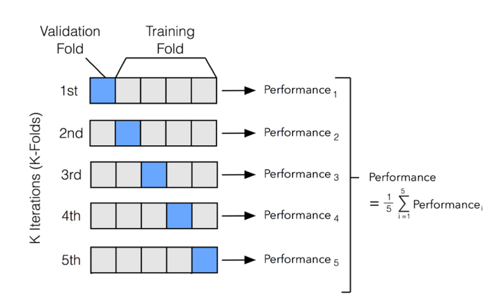
- Partition once into \(K\) folds; each fold is the validation set exactly once; average the \(K\) scores.
- Every point is tested once and trained on \(K-1\) times — nothing wasted, no lucky split.
- Larger \(K\): more training data per fit, more fits to run; \(K = n\) is leave-one-out.
The full protocol: lock away a test set → choose the hyperparameter by CV on the rest → refit on all training data → score the test set once. That last number is the only one you may report.
What the lecture did not draw: learning curves
The plots so far vary the model at fixed data. Today’s stretch holds the model fixed and varies the amount of data:
High bias (a line on a cubic)
- train and validation error converge fast
- … to a level well above the noise floor
- more data changes nothing
High variance (degree 12 on 10 points)
- training error ≈ 0, validation error large
- a gap that narrows only as \(n\) grows
- more data helps — and so would a simpler model
Learn to read the two signatures, then diagnose a mystery model from its curve alone and prescribe the fix: more data, a simpler model, or a more flexible one.
Going deeper
Full lecture notes: Generalization: Why Training Error Lies
- The Supervised Contract — the i.i.d. assumption and when it fails
- A Toy Example: Polynomial Curve Fitting — the \(k = 0, 1, 3, 9\) fits
- Generalization Error — the train-vs-test curve; Overfitting — why, and three fixes
- Bias and Variance and the Bias-Variance Trade-Off
- Parameters and Hyperparameters; Holding Out Data; Grid Search
- \(K\)-Fold Cross-Validation and Hold Out Strategies
- How This Plays Out This Term — the same trade-off, a different knob each week
Reminder: quiz 1 is one week out
Wed Oct 7, in class — closed notes, paper and pencil, covering lectures 01–07 (foundations thru today).
- The reference sheet for the unit is published today: quiz1-reference.pdf. Study with it — the printed copy handed out on quiz day is identical, and it is the only sheet allowed in the room.
- Today’s ideas that live on the sheet: the contract, overfitting, bias vs variance, hold-out / \(K\)-fold CV.
- The homework sets and knowledge checks are the practice; the recap decks are the answer keys.
In-Class Activity
Activity: train/test discipline, then learning curves
Goal: on your section’s synthetic regression, reproduce the train-vs-test curve for degrees 0–12 and pick the degree; pick it again with 5-fold CV without touching the test set; measure bias and variance for \(k = 1\) vs \(k = 9\) by refitting on many samples; then draw learning curves for an under-fit and an over-fit model and diagnose a mystery model from its curve.
- Work in groups of 2–3. Open your section’s notebook.
- Parts marked (autograded) are submitted to Gradescope; the rest is participation.
- Staff will circulate — be ready to explain any part of your work.
- Dependencies:
numpy,matplotlib,scikit-learn.


The activity notebook goes live on the day of the lecture. Colab is optional — you can also open it on GitHub and run it locally.