Recap: Probabilistic Modeling
DS701 Session 6 — Wed Sep 23, 2026


Today’s plan
- 5 min — knowledge-check review
- 20 min — highlights and Q&A (answer or pass — answering always earns credit)
- 60 min — in-class activity (small groups): fit, check, then simulate
- wrap-up and cold-call check-ins
Knowledge-Check Review
KC 1: The recipe, twice
The lecture fits a probability model to data in the same four steps twice — for Boston July temperatures and for the Prussian horse-kick counts. List the four steps, and for each dataset name the distribution family chosen and give one phrase saying why that family fits the shape of the data.
Show answer
Answer. (1) Look at the data and pick a family whose shape matches; (2) estimate the parameters; (3) check the fit; (4) use the model.
- July temperatures → Gaussian: continuous, unimodal, symmetric, bell-shaped.
- Horse-kick deaths per corps-year → Poisson: small non-negative counts of rare events at a roughly constant rate — a bell is the wrong shape for \(0, 1, 2, \dots\)
KC 2: What “maximum likelihood” means
In one or two sentences, what does it mean for \(\hat\mu\) and \(\hat\sigma^2\) to be the maximum likelihood estimates of a Gaussian’s parameters, and what do those estimates turn out to be? Why does maximizing the log-likelihood give the same answer as maximizing the likelihood?
Show answer
Answer. The MLE is the parameter setting that makes the observed data most probable — it maximizes \(L(\mu,\sigma^2) = \prod_n \mathcal{N}(x_n \mid \mu, \sigma^2)\) (a product because the samples are independent).
Setting the derivatives of \(\ell = \log L\) to zero gives
\[ \hat\mu = \frac{1}{N}\sum_{n=1}^N x_n, \qquad \hat\sigma^2 = \frac{1}{N}\sum_{n=1}^N (x_n - \hat\mu)^2 \]
— the “natural choice” from the first part of the lecture is the MLE.
\(\log\) is monotonically increasing, so the argmax of \(\log L\) is the argmax of \(L\); the log turns the product into a sum, which is easier to differentiate and numerically better behaved.
KC 3: Reading a confidence interval
From 2,821 July days the lecture reports a 95% confidence interval for the mean July temperature of \([23.12, 23.35]\) °C, with \(\hat\mu = 23.2\) °C and \(\hat\sigma = 3.2\) °C. A friend reads this as “so 95% of July days in Boston are between 23.12 and 23.35 °C.” Explain what is wrong with that reading, and use the two fitted numbers to say roughly what range does contain about 95% of individual July days.
Show answer
Answer. The interval is about the uncertainty in the mean, not the spread of days. Its half-width is \(1.96 \times s/\sqrt{n} \approx 1.96 \times 3.2/\sqrt{2821} \approx 0.12\) °C, and it shrinks like \(1/\sqrt{n}\) — day-to-day variation does not shrink at all.
Individual days are described by the fitted Gaussian itself: about 95% of July days fall within \(\hat\mu \pm 2\hat\sigma \approx 23.2 \pm 6.4\), i.e. roughly 17–29.5 °C.
And “95%” is a property of the procedure — 95% of intervals built this way cover the true mean — not a probability statement about this one interval. You will see this in today’s activity.
Highlights
Idea 1 — fit, then check
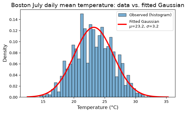
Fitting is cheap. Checking is what makes it a model rather than an assumption.
- Overlay the fitted density on the histogram.
- Compare what the model predicts with what you count: within \(1\sigma\): model \(0.683\), data \(0.664\); within \(2\sigma\): \(0.954\) vs \(0.966\).
- Test an implied property: for a Poisson, mean \(=\) variance (\(0.610\) vs \(0.608\)).
- Then use it: \(P(T > 30\,°\text{C})\) — model \(0.0165\), data \(0.0117\). Least trustworthy in the tails.
Idea 1, continued — when the check fails, believe the check
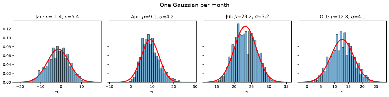

- One Gaussian per month: parameters differ a lot, and April shows a warm tail the bell cannot follow. The check tells you where the model is trustworthy.
- Horse kicks: \(\hat\lambda = 0.61\) deaths per corps-year predicts \(108.7 / 66.3 / 20.2 / 4.1 / 0.6\) corps-years with \(0/1/2/3/4\) deaths; observed \(109 / 65 / 22 / 3 / 1\).
- So the years with 3 or 4 deaths are exactly what randomness looks like at a constant rate — no story needed.
Idea 2 — MLE: maximize the likelihood of what you saw
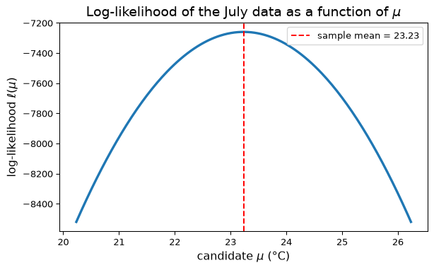
The Gaussian log-likelihood of the July data as \(\mu\) varies (\(\sigma\) fixed) — it peaks exactly at the sample mean.
The recipe, for any model:
- Write the probability of the observed data as a function of the parameters (independence \(\Rightarrow\) a product).
- Take the log (product \(\to\) sum; same argmax).
- Maximize: set derivatives to zero.
\[ \ell(\mu,\sigma^2) = -\tfrac{N}{2}\log(2\pi\sigma^2) - \tfrac{1}{2\sigma^2}\textstyle\sum_n (x_n-\mu)^2 \] \[ \frac{\partial \ell}{\partial \mu} = \frac{1}{\sigma^2}\sum_n (x_n-\mu) = 0 \;\Rightarrow\; \hat\mu = \frac{1}{N}\sum_n x_n \]
Idea 2, continued — the same recipe, and where you will meet it again
- Gaussian: \(\hat\mu = \frac{1}{N}\sum_n x_n\), \(\;\hat\sigma^2 = \frac{1}{N}\sum_n (x_n-\hat\mu)^2\) (divide by \(N\); pandas’
.std()uses \(N-1\) — negligible for large \(N\)). - Poisson: \(\ell(\lambda) = \log\lambda \sum_n k_n - N\lambda - \sum_n \log k_n!\), so \(\hat\lambda = \frac{1}{N}\sum_n k_n\) — the sample mean count.
- Multivariate Gaussian: the sample mean vector and sample covariance matrix —
df.mean(),df.cov().
You will see MLE again — twice.
- Next lecture: Gaussian Mixture Models maximize a likelihood where several Gaussians’ parameters are unknown at once and no closed form exists \(\Rightarrow\) Expectation–Maximization.
- Later: logistic regression is MLE for a model of class probabilities.
Idea 3 — covariance shapes the multivariate Gaussian
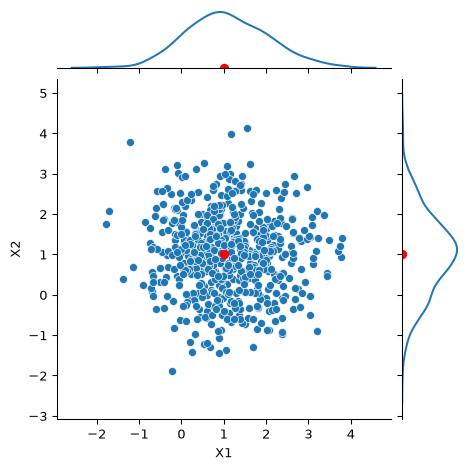
\(\Sigma = \begin{bmatrix}1&0\\0&1\end{bmatrix}\)
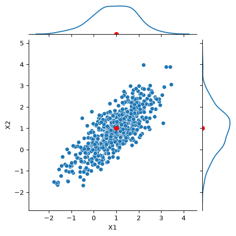
\(\Sigma = \begin{bmatrix}1&0.8\\0.8&1\end{bmatrix}\)
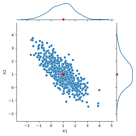
\(\Sigma = \begin{bmatrix}1&-0.8\\-0.8&1\end{bmatrix}\)
- \(\mathbf{X} \sim \mathcal{N}(\mathbf{\mu}, \Sigma)\): same two parameters as before, except the mean is a vector and the variance is a matrix, \(\Sigma_{ij} = \text{Cov}(X_i, X_j)\).
- \(\text{Cov}(X,Y) = E[(X-\mu_X)(Y-\mu_Y)]\); correlation \(\rho = \text{Cov}/(\sigma_X\sigma_Y) \in [-1,1]\). \(\rho = 0\) means no linear relationship — not independence.
- The off-diagonal stretches circles into tilted ellipses; the marginals stay Gaussian. (TSLA/NVDA: \(\rho \approx 0.86\) — a cloud along the diagonal, and arguably not one Gaussian. Hold that thought for GMMs.)
Idea 4 — the CLT: sample means become Gaussian, and narrow
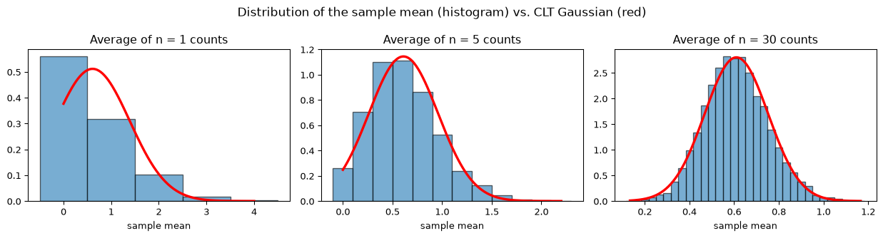
- Average \(n\) horse-kick counts (definitely not Gaussian), repeat 5000 times, histogram the averages.
- Any distribution with finite variance: as \(n\) grows the sample mean is \(\approx \mathcal{N}(\mu, \sigma^2/n)\).
- Two things happen at once: the shape becomes a bell, and the spread shrinks — the standard error is \(\sigma/\sqrt{n}\).
Idea 4, continued — a confidence interval, and how to read it
\[ \bar{x} \;\pm\; z_{1-\alpha/2}\,\frac{s}{\sqrt{n}}, \qquad z_{0.975} \approx 1.96 \]
- All July days (\(n = 2821\)): \([23.12,\ 23.35]\) °C. July 2020 alone (\(n = 31\)): \([22.83,\ 25.28]\) °C.
- The 95% is about the procedure: repeat the experiment many times and about 95% of the intervals cover the true mean. Any particular interval either does or does not.
- Width \(\propto 1/\sqrt{n}\): to halve it you need four times the data.
- It quantifies uncertainty in the mean only — individual days still range over \(\mu \pm 2\sigma\).
- Assumes independent samples; hot days cluster, so the honest interval is a bit wider.
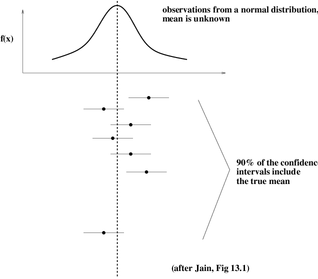
Each bar is the interval from one dataset; most cover the true mean, a few miss.
In-Class Activity
Activity: fit, check — then simulate what the theorems promise
Goal: run the recipe yourself on a month of Boston temperatures (Gaussian, MLE by hand and with scipy) and on the horse-kick counts (Poisson), check each fit and use it — then, as the stretch, treat your fitted Poisson as a known population and watch the Law of Large Numbers, the Central Limit Theorem, and the coverage of your own 95% confidence intervals.
- Work in groups of 2–3. Sections A1 and B1 get different months, corps, and seeds — open your section’s notebook.
- Parts marked (autograded) are submitted to Gradescope; the rest is participation.
- Staff will circulate — be ready to explain any part of your work.
- Dependencies:
numpy,pandas,matplotlib,scipyonly.


The activity notebook goes live on the day of the lecture. Colab is optional — you can also open it on GitHub and run it locally.
Going deeper
Full lecture notes: Probabilistic Modeling: Fitting Distributions to Data
- Checking the Fit and Checking the Fit Quantitatively — the overlay and the \(\pm k\sigma\) fractions
- The Model: The Poisson Distribution — counts, and the observed-vs-predicted table
- Likelihood Function → Gaussian MLEs → The Same Recipe for the Poisson; full derivation in Appendix 05A
- Covariance, Correlation, The Multivariate Gaussian
- The Central Limit Theorem, The Standard Error, Reading a Confidence Interval Correctly
- Background: Probability and Statistics Refresher
- Next up: Gaussian Mixture Models and EM (06) — the same likelihood, several Gaussians at once.