Causal Inference: Estimating Effects (Optional Module)

Optional module

This module extends Lecture 14. It is not required: it goes deeper into material that Lecture 14 introduces.

Lecture 14 showed how to choose an adjustment set \(S\) with the backdoor criterion, and named the estimators and natural-experiment designs that use it. This module works those estimators on simulated data and looks at the designs in detail.

Causal graphs: a recap

From Lecture 14:

Every path is built from chains, forks and colliders. Chains and forks are open until you condition on them; colliders are closed until you do (or condition on a descendant).
A backdoor path starts with an arrow into \(X\). A set \(S\) satisfies the backdoor criterion if it blocks every backdoor path and contains no descendant of \(X\).
Then conditional ignorability holds, \(\{Y(0), Y(1)\} \perp\!\!\!\perp T \mid S\), and regression, stratification, matching or propensity scores can do the adjusting.

The running example: \(X\) = exercise, \(Y\) = heart health. When we turn to estimation, the treatment is called \(T\), as in Lecture 14’s potential-outcomes notation.

Worked example

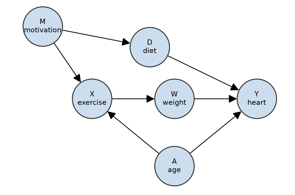
Back to the exercise DAG (\(X\) = exercise, \(Y\) = heart health):

\[ A \to X,\; A \to Y,\; M \to X,\; M \to D,\; D \to Y,\; X \to W,\; W \to Y \]

Paths from \(X\) to \(Y\): \(X \to W \to Y\); \(X \leftarrow A \to Y\); \(X \leftarrow M \to D \to Y\).
Causal path: \(X \to W \to Y\) — leave \(W\) alone.
Backdoor paths: \(X \leftarrow A \to Y\) (open, fork at \(A\)) and \(X \leftarrow M \to D \to Y\) (open, fork at \(M\), chain at \(D\)). No colliders anywhere.
Block the first with \(A\); block the second with \(M\) or \(D\).
Valid adjustment sets: \(\{A, M\}\), \(\{A, D\}\), or \(\{A, M, D\}\). Not \(\{A\}\) alone (leaves a backdoor open); not anything containing \(W\) (a descendant of \(X\)).

In regression terms: Y ~ X + A + M recovers the total effect of exercise; Y ~ X + A + M + W does not.

Regression adjustment on a simulation

A confounder \(Z\) (how sick a patient is) makes treatment more likely and makes the outcome worse. The true effect of \(T\) is \(3\).

Code

import numpy as np, pandas as pd, statsmodels.formula.api as smf

rng = np.random.default_rng(0)
n = 4000
Z = rng.normal(0, 1, n)                                         # sickness
T = (rng.uniform(size=n) < 1 / (1 + np.exp(-Z))).astype(int)   # sicker -> more likely treated
Y = 3.0 * T - 2.0 * Z + rng.normal(0, 1, n)                    # sicker -> worse; TRUE effect = 3.0
df = pd.DataFrame({"Y": Y, "T": T, "Z": Z})

naive = smf.ols("Y ~ T", data=df).fit().params["T"]
adj   = smf.ols("Y ~ T + Z", data=df).fit().params["T"]
print(f"True effect        = 3.00")
print(f"Naive (ignore Z)   = {naive:.2f}   <- biased")
print(f"Adjusted (+ Z)     = {adj:.2f}   <- recovers truth")

True effect        = 3.00
Naive (ignore Z)   = 1.33   <- biased
Adjusted (+ Z)     = 3.00   <- recovers truth

Predict the sign before you run it: \(Z\) raises treatment and lowers \(Y\), so the naive estimate is biased down. The treatment looks less than half as effective as it is, because the sickest were the ones treated.

Stratification: Lecture 14’s move on a continuous \(Z\)

Cut \(Z\) into strata, compare treated and control within each, then average with the population’s stratum shares — Lecture 14’s direct standardization, with \(S\) in place of kidney-stone size.

Code

def stratified(df, k):
    """Direct standardization over k equal-size strata of Z."""
    q = pd.qcut(df["Z"], k, labels=False)
    means = df.groupby([q, "T"])["Y"].mean().unstack()     # rows: strata, cols: T = 0, 1
    within = means[1] - means[0]                           # effect inside each stratum
    return within, (within * q.value_counts(normalize=True).sort_index()).sum()

for k in (5, 10, 20):
    print(f"{k:2d} strata: standardized effect = {stratified(df, k)[1]:.2f}")

 5 strata: standardized effect = 2.84
10 strata: standardized effect = 2.94
20 strata: standardized effect = 2.98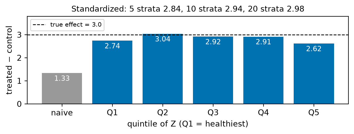

Coarse strata leave residual confounding inside each stratum; finer strata close the gap. Regression is the limit of infinitely fine strata — bought with a linearity assumption.

Propensity scores in one slide

When \(S\) is high-dimensional, matching directly is hard. Rosenbaum and Rubin showed it is enough to match or weight on the scalar propensity score \(e(S) = P(T{=}1\mid S)\) (Rosenbaum and Rubin 1983).

Code

from sklearn.linear_model import LogisticRegression

# Estimate propensity, then inverse-propensity weighting (IPW) for the ATE
ps = LogisticRegression().fit(df[["Z"]], df["T"]).predict_proba(df[["Z"]])[:, 1]
w = np.where(df["T"] == 1, 1 / ps, 1 / (1 - ps))
ate_ipw = (np.sum(w * df["T"] * df["Y"]) / np.sum(w * df["T"])
           - np.sum(w * (1 - df["T"]) * df["Y"]) / np.sum(w * (1 - df["T"])))
print(f"IPW estimate of ATE = {ate_ipw:.2f}   (true = 3.0)")

IPW estimate of ATE = 2.98   (true = 3.0)

Inverse-propensity weighting builds a “pseudo-population” in which treatment is unrelated to \(S\) — mimicking a randomized experiment from observational data.

Positivity: can we see it?

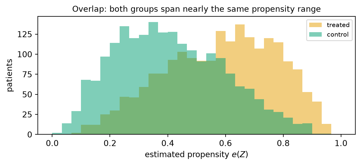
treated: e from 0.07 to 0.96;  control: 0.02 to 0.94;  largest weight = 15.5

If one histogram had mass where the other has none, some units would have no comparable counterpart. An \(e\) of \(0.01\) gives a weight of \(100\): a tight standard error around a number that means nothing.

Same adjustment set, same answer

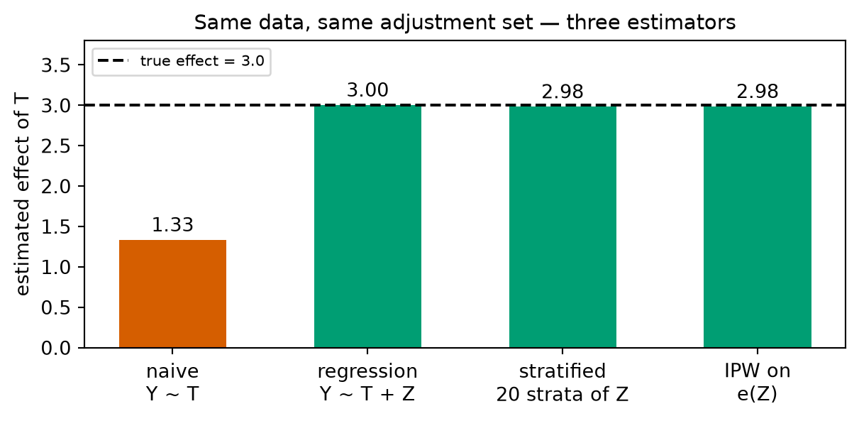
Identification (which \(S\)) and estimation (which estimator) are separate decisions. A wrong \(S\) gives a wrong answer with a tight standard error — no estimator rescues a bad graph.

When confounders are unobserved: natural experiments

Adjustment only works for confounders we can measure. When we can’t, we look for “nature’s randomization” — sources of variation in treatment that are as good as random (Angrist and Pischke 2014).

Three workhorse designs:

Difference-in-Differences (DiD),
Instrumental Variables (IV),
Regression Discontinuity (RD).

Difference-in-Differences

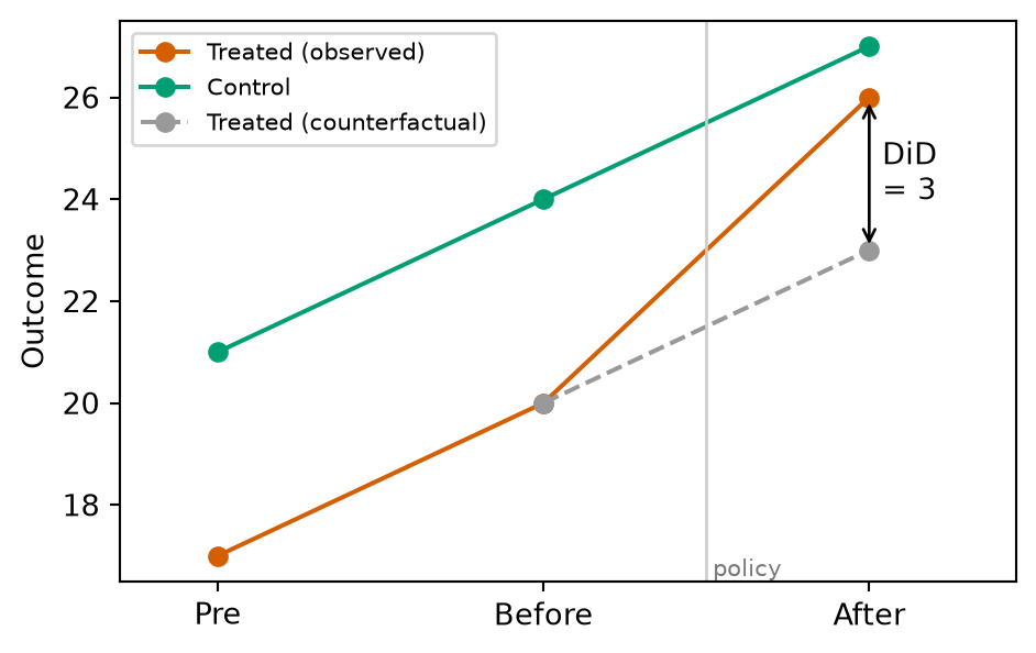
Compare the change in a treated group to the change in a control group over time. This differences out any fixed differences between the groups.

	Before	After	Change
Treated	20	26	+6
Control	24	27	+3

DiD \(= (26 - 20) - (27 - 24) = \mathbf{3}\).

Key assumption: parallel trends — absent treatment, both groups would have moved together. The only check you can run is on the pre period: here both rose by 3.

Card and Krueger used DiD to show that a New Jersey minimum-wage increase did not reduce fast-food employment relative to neighboring Pennsylvania (Card and Krueger 1994).

Instrumental variables & regression discontinuity

Instrumental variable (IV)

An instrument \(L\) shifts the treatment and affects the outcome only through it:

\[ L \rightarrow T \rightarrow Y, \quad L \not\rightarrow Y \text{ directly}. \]

Vietnam draft lottery as an instrument for military service.
Distance to college as an instrument for years of schooling.

\(L\) acts like the coin flip we wish we had run.

Lecture 14’s instrument in graph terms states its three conditions as a DAG.

Regression discontinuity (RD)

Treatment switches on at a cutoff of a running variable. Units just above vs. just below are comparable.

Scholarship awarded at a test-score threshold.
Class-size caps that trigger a new section.

Compare outcomes in a narrow window around the cutoff.

Three designs, three assumptions

Design	As-good-as-random variation	Assumption	How it fails
DiD	the change in treated vs. control	parallel trends	pre-period trends already diverge
IV	an instrument \(L\)	relevance (\(L \to T\)), exclusion (no \(L \to Y\)), independence (no backdoor \(L\)–\(Y\))	the lottery shifts earnings via draft avoidance (staying in college)
RD	a cutoff on a running variable	nothing else jumps at the cutoff; no precise manipulation	people bunch just above the threshold

Each design swaps “no unmeasured confounders” for a different, often more credible, assumption that data cannot fully verify. No free lunch.

Assumptions you can’t skip

Every observational causal estimate relies on assumptions (Hernán and Robins 2020):

Conditional ignorability — \(\{Y(0),Y(1)\} \perp\!\!\!\perp T \mid S\): the adjustment set blocks every backdoor path. The DAG argues it; data cannot check it.
Positivity (overlap) — every unit has a nonzero chance of each treatment (\(0 < e(S) < 1\)).
SUTVA — the assumption Lecture 14’s switching equation \(Y^{\text{obs}} = T\,Y(1) + (1-T)\,Y(0)\) quietly made: one unit’s treatment doesn’t affect another’s outcome, and there is only one version of “treated.”
Correct graph — the DAG reflects reality.

Since ignorability is untestable, good practice includes a sensitivity analysis: how strong would an unmeasured confounder have to be to overturn the conclusion?

Tools and the modern workflow

DoWhy — model (DAG) → identify → estimate → refute; a clean four-step API (Sharma and Kiciman 2020).
EconML — ML-based heterogeneous treatment effects (CATE).
dagitty — draw a DAG in the browser; it tells you the valid adjustment sets.
Classical estimators live in statsmodels, scikit-learn, and linearmodels.

The workflow is always: draw the graph → identify an estimand → estimate → challenge it with robustness checks. The graph comes first.

Summary

A causal DAG encodes your assumptions, not the data’s. Nodes are variables, arrows are direct causes, and every path is built from chains, forks, and colliders.
Chains and forks are open until you condition on them; colliders are closed until you do (or condition on a descendant). A path transmits association only if it is open.
The backdoor procedure sorts every path into causal, backdoor or neither, then blocks every open backdoor with non-descendants of \(X\) — never a mediator, never a collider.
Identification first, estimation second: given a valid \(S\), regression, stratification and IPW agree; with a wrong \(S\) none of them can help.
When confounders are unmeasured, use natural experiments — DiD (parallel trends), IV (relevance, exclusion, independence), RD (nothing else jumps at the cutoff) — and state the standing assumptions (ignorability, positivity, SUTVA).

Practice scenarios (self-check)

For each scenario, draw the DAG, name the confounder, the tempting-but-wrong control (a mediator or collider), and a design you would use. Then open the intended answers.

A. Product / tech. Does adding a “free shipping” badge on product pages increase purchases? You have historical logs; badges were shown more often on popular items.

B. Health. Does a new fitness-tracking app reduce users’ resting heart rate? People who download it are already more health-conscious.

C. Education. Does an optional tutoring program raise final grades? Students self-select into tutoring, and struggling students are more likely to sign up.

D. Policy. Does a city’s new bike-lane network reduce traffic accidents? It was built in denser, wealthier neighborhoods first.

Intended answers

A. Confounder: item popularity (drives both the badge and purchases). Tempting control: “add-to-cart” — a mediator on badge → add-to-cart → purchase. Design: an A/B test that randomizes the badge, or adjust for popularity with a propensity score.
B. Confounder: health-consciousness. Tempting controls: steps per day (a mediator — the app works by getting people moving) and “posted an app review” (a collider — caused by both installing the app and by feeling the benefit). Design: randomize a free premium tier as an encouragement (an instrument), or DiD on users’ heart rate before and after installing.
C. This is Lecture 14’s tutoring DAG. Confounder: prior GPA (struggling students sign up and score lower, so the naive estimate is biased down). Tempting controls: study hours (mediator) and honor roll (collider). Design: adjust for prior GPA; or RD if tutoring is assigned below a GPA cutoff.
D. Confounder: neighborhood density / wealth. Tempting control: cyclist volume — a mediator (lanes → more cyclists → accidents). Design: DiD comparing accident trends in neighborhoods that got lanes early vs. late, checking pre-period trends.

References

Causal Inference: What If — Hernán & Robins (free PDF)
Causal Inference: A Primer — Pearl, Glymour & Jewell
“A Crash Course in Good and Bad Controls” — Cinelli, Forney & Pearl
DoWhy documentation and dagitty.net

Bibliography

Angrist, Joshua D., and Jörn-Steffen Pischke. 2014. Mastering ’Metrics: The Path from Cause to Effect. Princeton University Press.

Card, David, and Alan B. Krueger. 1994. “Minimum Wages and Employment: A Case Study of the Fast-Food Industry in New Jersey and Pennsylvania.” American Economic Review 84 (4): 772–93.

Hernán, Miguel A., and James M. Robins. 2020. Causal Inference: What If. Chapman & Hall/CRC. https://www.hsph.harvard.edu/miguel-hernan/causal-inference-book/.

Rosenbaum, Paul R., and Donald B. Rubin. 1983. “The Central Role of the Propensity Score in Observational Studies for Causal Effects.” Biometrika 70 (1): 41–55. https://doi.org/10.1093/biomet/70.1.41.

Sharma, Amit, and Emre Kiciman. 2020. DoWhy: An End-to-End Library for Causal Inference. https://arxiv.org/abs/2011.04216.