Recap: Logistic Regression
DS701 Session 13 — Mon Oct 19, 2026


Today’s plan
- 5 min — knowledge-check review
- 20 min — highlights and Q&A (answer or pass — answering always earns credit)
- 40 min — case study: the credit union’s approval threshold
- wrap-up and cold-call check-ins
Knowledge-Check Review
KC 1: The model, in one line
Write down the logistic regression model: what linear function does it fit, what quantity is that linear function equal to, and how do you get from it to a probability \(p(y{=}1 \mid x)\)? Then say how the coefficients are chosen (which principle) and why, unlike linear regression, they cannot be found in closed form.
KC 2: A coefficient is an odds ratio
In the admissions fit, \(\hat\beta_{\text{gpa}} = 0.777\). A classmate reads this as “one more GPA point raises the probability of admission by 0.777”. What does the coefficient actually say, what does \(e^{0.777} \approx 2.17\) mean, and why is there no single change in probability?
KC 3: 0.5 is not a law of nature
To turn logistic regression into a classifier the lecture used the rule “say yes if \(p(y{=}1 \mid x) > t\)” and found on the admissions data that F1 peaked near \(t \approx 0.35\), not \(0.5\). Explain what lowering the threshold does to precision and to recall, why \(0.5\) is not automatically the right choice, and give one real setting where you would deliberately pick a low threshold and one where you would pick a high one.
Highlights
Logistic regression = a linear model + a sigmoid
Last lecture: a continuous \(y\) as a linear function of \(x\). Today: a 0/1 \(y\), and we want a probability.
- A line takes values in \((-\infty,\infty)\); a probability lives in \([0,1]\). So fit the line to something unbounded: the log-odds \(\log\frac{p}{1-p}\) (the logit).
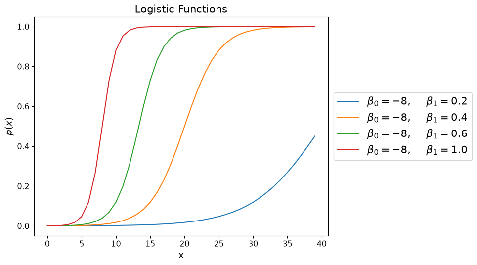
- Sigmoid: \(p(y{=}1 \mid x) = \sigma(\beta_0 + \beta_1 x)\).
- \(\beta_1\) sets the steepness (and direction); \(\beta_0\) shifts the curve; \(p = 0.5\) at \(x = -\beta_0/\beta_1\); \(\beta_0\) is the log-odds at \(x = 0\) — the base rate only if the features are centred (admissions: \(\sigma(\hat\beta_0) = 3\%\) vs 32% admitted).
- Read a coefficient as in linear regression — but on the log-odds scale: \(e^{\beta_1}\) multiplies the odds per unit of \(x\) (GPA: \(\times 2.2\) per point).
Fit by maximum likelihood — same principle as Lecture 05
One observation: \(\;\text{P}(y_i \mid x_i) = p_i^{\,y_i}\,(1-p_i)^{1-y_i}, \qquad p_i = \sigma(\boldsymbol{\beta}^\top\mathbf{x}_i).\)
- Data are independent, so the likelihood is the product; the log-likelihood is the sum \(\;\ell(\boldsymbol{\beta}) = \sum_i \big[y_i\log p_i + (1-y_i)\log(1-p_i)\big].\)
- In Lecture 05 you maximized likelihoods for a Poisson and a Gaussian and got a formula. Linear regression is the lucky case: Gaussian noise ⇒ MLE = least squares ⇒ closed form.
- Here there is no closed form. Gradient ascent: \(\boldsymbol{\beta}^{(t+1)} = \boldsymbol{\beta}^{(t)} + \alpha\,\nabla\ell(\boldsymbol{\beta}^{(t)})\), with the tidy gradient \(\nabla\ell = X^\top(\mathbf{y} - \mathbf{p})\) — residual times feature, just like the normal equations, with a sigmoid inside.
statsmodels.Logit/sklearn.LogisticRegressiondo the climb for you and give a coefficient per feature (plus the column of ones for \(\beta_0\)).
Today’s activity, Part 1: you write \(\sigma\), \(\ell\), and one gradient step by hand — then check that sklearn lands in the same place.
The boundary is still a line
- “Assign to class 1 if \(p(y{=}1 \mid x) > 0.5\)” \(\iff\) log-odds \(> 0\) \(\iff\) \(\boldsymbol{\beta}^\top\mathbf{x} > 0\).
- The sigmoid is monotone, so the decision depends only on the sign of the linear score — the boundary is a hyperplane. The nonlinearity lives in the confidence, not the boundary.
- Any other threshold \(t\) just slides the plane parallel to itself, to \(\boldsymbol{\beta}^\top\mathbf{x} = \log\frac{t}{1-t}\).
- Once you classify, you owe an evaluation. Four outcomes: TP, FP, FN, TN, and two rates that pull in opposite directions: \[ \text{Precision} = \frac{TP}{TP+FP}, \qquad \text{Recall} = \frac{TP}{TP+FN}, \qquad F_1 = \frac{2PR}{P+R}. \]
Evaluation beyond accuracy
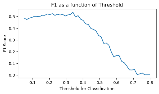
Admissions: F1 peaks near \(t \approx 0.35\) — the model rarely says “admit” at 0.5 because admits are the minority (and “always reject” is already 68% accurate).
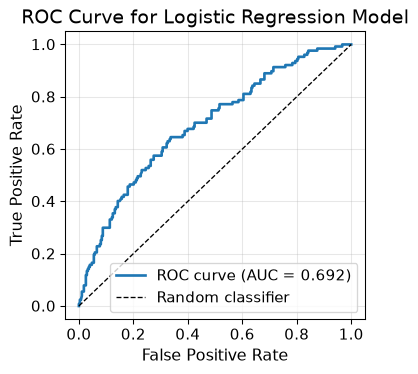
ROC: TPR vs FPR, one point per threshold; diagonal = random; AUC summarizes ranking quality without choosing a threshold (0.71 on the held-out split).
The threshold is a decision
AUC tells you how good the scores are. It does not tell you where to cut.
- False positive costs \(C_{FP}\), false negative \(C_{FN}\). Say “yes” when \(p\,C_{FN} > (1-p)\,C_{FP}\): \[ p > t^* = \frac{C_{FP}}{C_{FP} + C_{FN}}. \]
- A miss four times as costly as a false alarm: \(t^* = 0.2\). Equal costs give back \(0.5\) — the only case where \(0.5\) is “right”.
class_weight="balanced"re-weights the fit so both classes count equally — a cost ratio set by the class frequencies, not by what the mistakes actually cost.
Today’s case study ends on exactly that cut: the lending desk’s approval threshold, from the costs they state.
Where this goes next
- Lecture 11B — Regularization (Wed): what goes wrong when the features are nearly redundant (coefficients blow up), and the fix — a penalty on the size of \(\boldsymbol{\beta}\), for linear and logistic regression.
- You have already met it without noticing:
sklearn’sLogisticRegression()penalizes by default, withC\(= 1/c\). 11B explains what that knob does. - And the threshold question comes back every time a model outputs a probability.
In-Class Activity
Activity — Case Study 11A: Setting the Approval Threshold for a Credit Union’s Small-Business Loans
The client: a Massachusetts credit union’s small-business lending desk.
- Can we get a repayment score we can see inside, not a black box?
- Which applications should be approved automatically — where do we cut?
The data: a simulator of the desk’s applicants, whose true answer you know
- Member records cannot be shared — this is a prototype until they can be
Activity — The Parts
- Build it: sigmoid and log-likelihood by hand, one gradient step; check against sklearn and draw the boundary it puts through the applicants
- The threshold decision: precision / recall / F1 across thresholds, ROC-AUC on a held-out split, and the cost-optimal \(t^* = C_{FP}/(C_{FP}+C_{FN})\) against \(0.5\) and
class_weight="balanced"
Report out: a two-sentence memo to the desk — which threshold, and the one caveat they must hear.
Activity — Logistics
- Work in groups of 2–3. Open your section’s notebook.
- Parts marked (autograded) are submitted to Gradescope; the rest is participation.
- Staff will circulate — be ready to explain any part of your work.
- Dependencies:
numpy,pandas,matplotlib,scikit-learn.


The activity notebook goes live on the day of the lecture. Colab is optional — you can also open it on GitHub and run it locally.
Going deeper
Full lecture notes: Logistic Regression
- Odds and Log-Odds — the logit, the sigmoid, what \(\beta_0\) and \(\beta_1\) do to the curve; Reading the coefficients as odds ratios
- Logistic vs Linear Regression — the likelihood, and why there is no closed form
- From one observation to the whole data set — the log-likelihood and its gradient \(X^\top(\mathbf{y}-\mathbf{p})\); Gradient ascent with a hand-computed step
- The decision boundary is still a hyperplane — drawn on the admissions data
- Logistic Regression in Perspective — accuracy vs prevalence, precision, recall, F1 vs threshold, and the cost-optimal threshold
- ROC-AUC Curve
- Next: Regularization (Lecture 11B)
- Background: MLE in Probabilistic Modeling; least squares in Linear Regression