Recap: Causal Inference
DS701 Session 18 — Wed Nov 4, 2026


Today’s plan
- 5 min — knowledge-check review
- 20 min — highlights and Q&A (answer or pass — answering always earns credit)
- 60 min — case study: did the community-health-worker program reduce ER visits
- wrap-up and cold-call check-ins
Causal inference is examined on quiz 3 (Wed Dec 2), and HW9 (released Mon Nov 9) rehearses it by hand. Today is not quiz review; use office hours for that.
Knowledge-Check Review
KC 1: The selection-bias term
The lecture decomposed the naive difference in means, \(\mathbb{E}[Y \mid T{=}1] - \mathbb{E}[Y \mid T{=}0]\), into a causal part plus a selection-bias term. In words, what does the selection-bias term measure, why is it nonzero in the hospital-visits example, and why does randomly assigning \(T\) make it zero?
KC 2: Three building blocks
Name the three elementary structures every path in a causal DAG is built from, and for each say (i) what the middle node is called and (ii) whether the path through it is open or blocked by default, and what happens when you condition on that middle node.
KC 3: “Controlling for more can only help”
In the tutoring example, \(X\) = tutoring and \(Y\) = final grade, with \(\text{GPA}_{\text{prior}} \to X\), \(\text{GPA}_{\text{prior}} \to Y\), \(X \to \text{Hours} \to Y\) and \(X \to \text{HonorRoll} \leftarrow Y\). A colleague argues that adjusting for \(\{\text{GPA}_{\text{prior}}, \text{Hours}, \text{HonorRoll}\}\) must be at least as good as adjusting for \(\{\text{GPA}_{\text{prior}}\}\) alone, “because controlling for more can only help.” Using the backdoor procedure, explain why the colleague is wrong about the total effect of tutoring — say what each of Hours and HonorRoll does to the estimate.
Highlights
1. A regression coefficient is an association, not an effect
OLS estimates \(P(Y \mid X)\); a causal claim is about \(P(Y \mid do(X))\), and the two differ whenever there is confounding.
Prediction — seeing
\[ P(Y \mid X = x) \]
“Among people I observe with \(X = x\), what is \(Y\)?”
Every model in this course so far.
Intervention — doing
\[ P(Y \mid do(X = x)) \]
“If I set \(X = x\) for everyone, what is \(Y\)?”
What a decision-maker needs.
The hospital model is a good predictor (“I see a visit, I predict higher mortality”) and a catastrophic guide to action (“close the hospitals”). Same table, two readings — the whole lecture is about the gap between them.
2. A confounder is a common cause
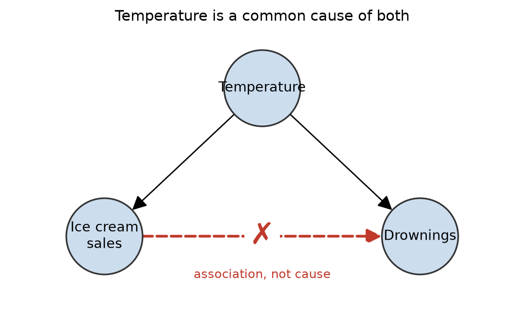
drownings ~ ice_cream: slope \(+0.032\), \(p \approx 0\) — every Lecture 10 diagnostic happy. Truth: zero (ice cream is not in the equation for drownings).drownings ~ ice_cream + temp: slope \(-0.007\). Adding the confounder = holding temperature fixed.- Which variables to add is a causal question the fitting procedure cannot answer. Unmeasured temperature → no model selection saves you.
Confounding is one of five ways to get an association: \(X \to Y\), reverse causation, a common cause, collider bias, or pure chance. Only the first is the effect the headline wants.
3. Naive difference \(=\) effect \(+\) bias
Potential outcomes \(Y(1), Y(0)\) define the effect, \(\tau_i = Y_i(1) - Y_i(0)\); you only ever observe one, so we target averages: \(\text{ATE} = \mathbb{E}[Y(1) - Y(0)]\), \(\text{ATT} = \mathbb{E}[Y(1) - Y(0) \mid T{=}1]\).
\[ \underbrace{\mathbb{E}[Y(1)\mid T{=}1] - \mathbb{E}[Y(0)\mid T{=}0]}_{\text{naive difference}} = \underbrace{\text{ATT}}_{\text{causal}} + \underbrace{\mathbb{E}[Y(0)\mid T{=}1] - \mathbb{E}[Y(0)\mid T{=}0]}_{\text{selection bias}} \]
Tutoring table. Every student gains exactly \(\tau_i = 2\), but the weaker three signed up. Observed: \(67 - 70 = -3\). Decomposed: ATT \(= 2\), bias \(= 65 - 70 = -5\). Right arithmetic, wrong causal reading.
Randomization. A coin flip gives
\[ \{Y_i(0), Y_i(1)\} \perp\!\!\!\perp T_i \]
so the groups match on every trait, measured or not: bias term \(= 0\) and \(\text{ATT} = \text{ATE}\). No list of confounders needed — why an A/B test is the gold standard.
4. Simpson’s paradox: give both arms the same case mix
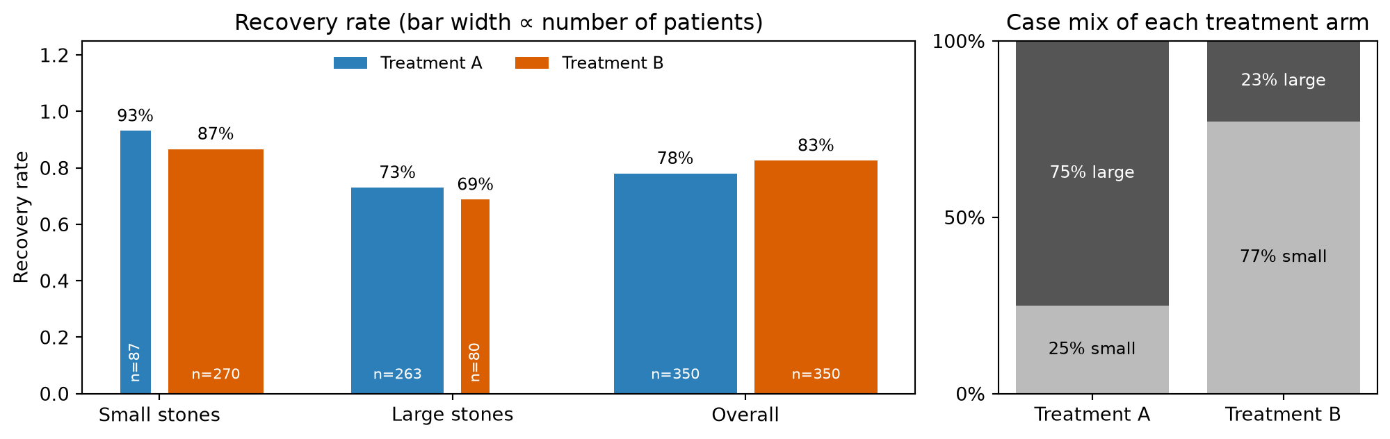
- A wins in every stratum; B wins overall. The confounder’s two fingerprints: the case mix differs between arms (75% vs. 23% large stones) and the strata differ in outcome.
- Direct standardization gives both arms the study’s case mix: \(P(Y \mid do(T{=}t)) = \sum_z P(Y \mid T{=}t, Z{=}z)\,P(Z{=}z)\) ⇒ A \(\approx 83\%\), B \(\approx 78\%\).
Y ~ T + Zis the regression form;Y ~ Talone is the naive difference. - Whether to adjust depends on the arrows, not the table — which is what the causal graph is for.
5. Adjust for forks — not mediators or colliders
| structure | middle node | adjust? | why |
|---|---|---|---|
| fork \(X \leftarrow Z \to Y\) | confounder | yes | blocks the backdoor path |
| chain \(X \to M \to Y\) | mediator | no* | it is the effect (overcontrol) |
| collider \(X \to C \leftarrow Y\) | collider | no! | conditioning creates association |
* unless you want the direct, not the total, effect.
So “throw every variable into the regression” is wrong. Today’s case study has you tell a health department which of its variables are the bad controls, and why.
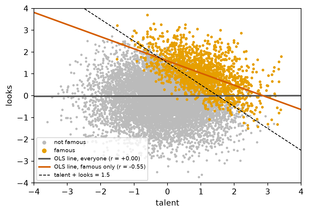
Talent and looks: independent by construction (corr \(\approx 0.00\)), yet among the famous corr \(\approx -0.55\) — selecting the famous conditions on the collider talent \(\to\) famous \(\leftarrow\) looks. Selecting on a descendant (follower count) does it too.
6. The backdoor criterion is a procedure
A backdoor path starts with an arrow into \(X\) — confounding in graph language. \(S\) is a valid adjustment set if it blocks every backdoor path and contains no descendant of \(X\).
- List every path from \(X\) to \(Y\), ignoring direction, visiting no node twice.
- Set aside the causal paths (all arrows away from \(X\)) — never block these.
- Classify the rest: first arrow into \(X\) → backdoor (mark open / blocked: forks & chains open, colliders closed); first arrow out of \(X\) but not causal (runs into a collider, \(X \to C \leftarrow Y\)) → neither, blocked as long as you leave \(C\) alone.
- Choose \(S\) blocking every open backdoor — a fork or chain node on each — with no collider or collider-descendant on any path and no descendant of \(X\).
- Report \(S\) — several may be valid; smallest is usually best.
KC 3 was this procedure on the tutoring DAG: only \(\{\text{GPA}_{\text{prior}}\}\) survives. Then — and only then — pick an estimator.
7. Identify first, then estimate
Confounders measured. Given a valid \(S\) (conditional ignorability: \(\{Y(0),Y(1)\} \perp\!\!\!\perp T \mid S\)), any of these recovers the effect:
- Regression — include \(S\), read the coefficient on \(T\).
- Stratification — direct standardization on \(S\).
- Matching on \(S\).
- Propensity score \(e(S) = P(T{=}1 \mid S)\) — match or weight on one number. Needs overlap: \(0 < e(S) < 1\).
A wrong \(S\) gives a wrong answer with a tight standard error.
Confounder unmeasured. Adjustment cannot block its backdoor. Look for as good as random variation — a natural experiment:
- DiD — change in treated vs. change in control; assumes parallel trends.
- RD — compare just above vs. just below a cutoff; assumes nothing else jumps there.
- IV, in graph terms: \(L \to T \to Y\), no arrow \(L \to Y\), nothing pointing into \(L\).
Every estimate rests on assumptions the data cannot verify — the graph itself, ignorability, overlap — so state them and run a sensitivity analysis: how strong would a hidden confounder have to be to overturn the conclusion?
Next session: we leave causal questions for prediction — neural networks: forward pass, loss, gradient descent, by hand.
In-Class Activity
Activity — Case Study 14: Did the Community Health Worker Program Reduce ER Visits?
Goal: a city public-health department ran a community-health-worker (CHW) program; its analysts say enrolled residents used the ER less, the budget office says more, and the commissioner wants to know whether the program caused anything before funding a second year.
- Part 1 — recompute the outcome table by neighborhood stratum, find the Simpson’s reversal and the confounder’s two fingerprints, and adjust it by direct standardization.
- Part 2 — trace the backdoor paths by hand on three candidate CHW DAGs, marking each open or blocked.
- Part 3 — propose one valid and one invalid adjustment set per DAG.
- Report out — a two-sentence memo to the commissioner: the recommendation and the one caveat, including what the department must not adjust for.
Work in groups of 2–3. Autograded questions are submitted to Gradescope; the discussion prompts and the memo are participation. Staff will circulate and ask for your memo, so agree on your answer.


The activity notebook goes live on the day of the lecture. Colab is optional — you can also open it on GitHub and run it locally.
Going deeper
Full lecture notes: Causal Inference
- What does a coefficient mean?, the ice cream regression, confounding and the hospital example
- Two different questions — \(P(Y \mid X)\) vs. \(P(Y \mid do(X))\); where spurious associations come from
- Potential outcomes, the all-seeing tutoring table, the fundamental problem, ATE and ATT, naive = ATT + selection bias
- Kidney stones, the two fingerprints, direct standardization, randomized experiments
- Reading a causal graph, the three building blocks, open and blocked paths, the golden rule
- The backdoor criterion, the procedure, by hand, the tutoring DAG answer
- Colliders and a collider’s descendants; mediators
- Four ways to adjust, natural experiments, an instrument in graph terms, assumptions you can’t skip
- Optional depth: the unscheduled module M14 — Estimating Causal Effects — estimator simulations, IPW, positivity, DiD and RD in detail