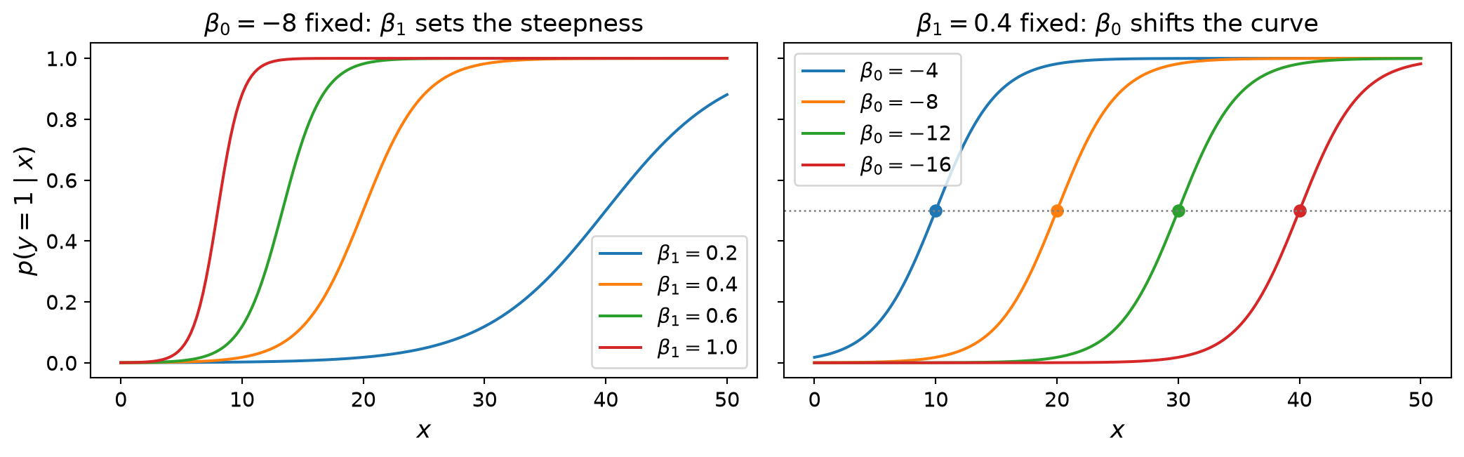
import numpy as npimport scipy as spimport matplotlib.pyplot as pltimport pandas as pdimport seaborn as snsimport matplotlib as mpimport sklearnfrom IPython.display import Image, HTMLimport statsmodels.api as smfrom sklearn import model_selectionfrom sklearn import metrics%matplotlib inline
So far we have seen linear regression: a continuous valued observation is estimated as a linear (or affine) function of the independent variables.
Today the observation is a 0/1 variable and we want a probability:
fit a linear model to the log-odds and invert it through the sigmoid,
fit the coefficients by maximum likelihood,
evaluate the result as a classifier, and choose its threshold.
Regularization – a penalty on the size of \(\boldsymbol{\beta}\), for linear and logistic regression alike – follows in Lecture 11B.
Estimating a Probability
Imagine that you are observing a binary variable – value 0 or 1.
That is, these could be pass/fail, admit/reject, Democrat/Republican, etc.
Assume there is some probability of observing a 1, and that probability is a function of certain independent variables.
So the key properties of a problem that make it appropriate for logistic regression are:
You are trying to predict a categorical variable
You want to estimate a probability of seeing a particular value of the categorical variable.
What is the probability I will be admitted to Grad School?
Let’s see how variables, such as,
GRE (Graduate Record Exam scores),
GPA (grade point average), and
prestige of the undergraduate institution
affect admission into graduate school.
The response variable, admit/don’t admit, is a binary variable.
So there are three predictor variables: gre,gpa and rank.
We will treat the variables gre and gpa as continuous.
The variable rank takes on the values 1 through 4 with 1 being the highest prestige.
NoteRank is ordinal, and we feed it in as a number
Treating rank as a number assumes that each step down in prestige has the same effect on the log-odds. The alternative is one indicator column per rank (C(rank) in formula syntax), which costs two more coefficients. We keep the numeric version here; the categorical version is shown in Appendix: Regression Formulas with statsmodels.
The first rows of the data (400 applicants), and some summary statistics:
Code
import os, urllib.requestdef data_file(path):"""Course data file: use a local copy (here, or in the repo root above a notebook in jupyter_notebooks/), else fetch it from the Materials repo (Colab)."""for prefix in ('', '../'):if os.path.exists(prefix + path):return prefix + path os.makedirs(os.path.dirname(path) or'.', exist_ok=True) urllib.request.urlretrieve('https://raw.githubusercontent.com/tools4ds/DS701-Materials-FA26/main/'+ path, path)return path# original data source: http://www.ats.ucla.edu/stat/data/binary.csvdf = pd.read_csv(data_file('data/ats-admissions.csv'))df.head(8)
admit
gre
gpa
rank
0
0
380
3.61
3
1
1
660
3.67
3
2
1
800
4.00
1
3
1
640
3.19
4
4
0
520
2.93
4
5
1
760
3.00
2
6
1
560
2.98
1
7
0
400
3.08
2
Code
df.describe().round(3)
admit
gre
gpa
rank
count
400.000
400.000
400.000
400.000
mean
0.318
587.700
3.390
2.485
std
0.466
115.517
0.381
0.944
min
0.000
220.000
2.260
1.000
25%
0.000
520.000
3.130
2.000
50%
0.000
580.000
3.395
2.000
75%
1.000
660.000
3.670
3.000
max
1.000
800.000
4.000
4.000
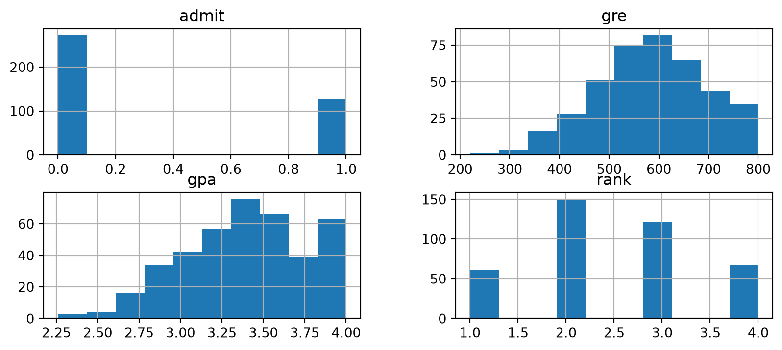
We can also plot histograms of the variables:
Code
df.hist(figsize = (10, 4));
Note how df.hist() automatically plots a histogram for each column in the dataframe as a subplot.
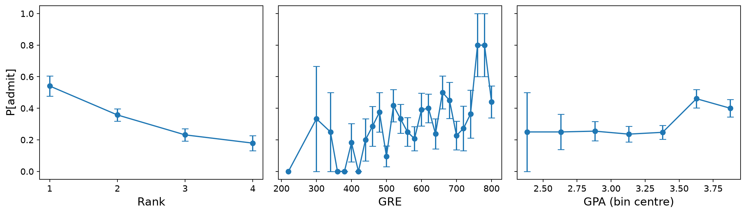
Mean admission rate against each feature, with standard-error bars:
For each value of a feature we plot the fraction of applicants admitted, and add error bars for the standard error of the mean. GPA takes almost as many values as there are applicants, so we aggregate it into 7 equal-width bins and plot each bin’s mean at the bin centre.
Note that there’s a greatly expanded groupby section in the Pandas refresher.
Code
def admit_rate(groups):"""Mean admission rate per group, with the standard error of the mean.""" grouped = groups['admit']return grouped.mean(), grouped.std() / np.sqrt(grouped.count())bins = np.linspace(df.gpa.min(), df.gpa.max(), 8)gpa_bin = pd.cut(df.gpa, bins, include_lowest=True)panels = [('Rank', admit_rate(df.groupby('rank'))), ('GRE', admit_rate(df.groupby('gre'))), ('GPA (bin centre)', admit_rate(df.groupby(gpa_bin, observed=True)))]fig, axs = plt.subplots(1, 3, figsize=(13, 3.8), sharey=True)for ax, (name, (means, errors)) inzip(axs, panels): x = [v.mid for v in means.index] if name.startswith('GPA') else means.index ax.errorbar(x, means, yerr=errors, marker='o', capsize=4) ax.set_xlabel(name, fontsize=14) ax.tick_params(labelsize=11)axs[0].set_xticks([1, 2, 3, 4])axs[0].set_ylabel('P[admit]', fontsize=14)plt.tight_layout()
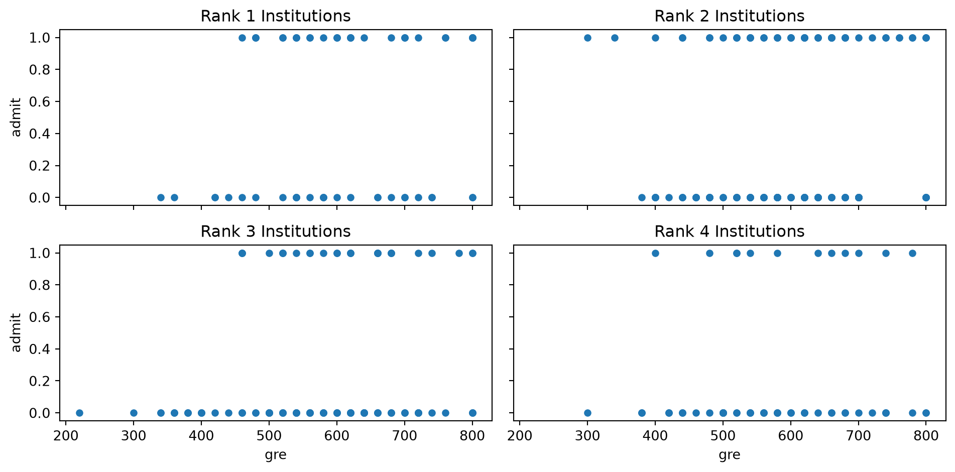
Finally, we plot admission status versus GRE score for each data point for each of the four ranks:
What we want to do is to fit a model that predicts the probability of admission as a function of these independent variables.
Logistic Regression
Logistic regression is concerned with estimating a probability.
However, all that is available are categorical observations, which we will code as 0/1.
That is, these could be pass/fail, admit/reject, Democrat/Republican, etc.
Now, a linear function like \(\beta_0 + \beta_1 x\) cannot be used to predict probability directly, because
the linear function takes on all values (from -\(\infty\) to +\(\infty\)),
and probability only ranges over \([0, 1]\).
Odds and Log-Odds
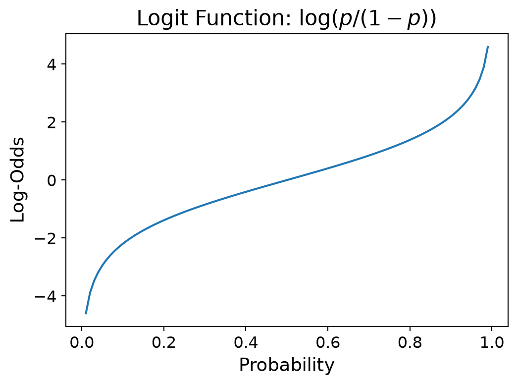
However, there is a transformation of probability that works: it is called log-odds.
For any probability \(p\), the odds is defined as \(p/(1-p)\), which is the ratio of the probability of an event to the probability of the non-event.
Notice that odds vary from 0 to \(\infty\), and odds < 1 indicates that \(p < 1/2\).
Odds are still not a good target for a linear function, for two reasons.
Range. A line takes negative values; odds cannot. Taking the log maps \((0, \infty)\) onto the whole real line, so nothing the line predicts is impossible.
Symmetry. Odds treat the two outcomes asymmetrically: \(p = 0.9\) gives odds \(9\) while \(p = 0.1\) gives odds \(1/9\). Log-odds are symmetric: \(+2.2\) and \(-2.2\). Swapping which outcome we call “1” just flips the sign of every coefficient.
It stretches the interval \((0, 1)\) onto the whole real line, with \(p = 1/2\) at \(0\): exactly the range a line can cover.
With \(d\) features we collect them, together with a leading \(1\) for the intercept, into \(\mathbf{x} = (1, x_1, \ldots, x_d)^T\) and the coefficients into \(\boldsymbol{\beta} = (\beta_0, \beta_1, \ldots, \beta_d)^T\). The model is then
Everything below is written for one feature; replace \(\beta_0 + \beta_1 x\) by \(\boldsymbol{\beta}^T\mathbf{x}\) and it holds for any number of features.
And again, in machine learning we just usually call this the sigmoid function, and denote it \(\sigma(z)\).
Logistic vs Linear Regression
Let’s take a moment to compare linear and logistic regression.
In Linear regression we fit
\[
y_i = \beta_0 +\beta_1 x_i + \epsilon_i.
\]
We do the fitting by minimizing the sum of squared errors \(\Vert\epsilon\Vert^2\). This can be done in closed form using either geometric arguments or by calculus.
Now, if \(\epsilon_i\) comes from a normal distribution with mean zero and some fixed variance, then minimizing the sum of squared errors is exactly the same as finding the maximum likelihood of the data with respect to the probability of the errors.
So, in the case of linear regression, it is a lucky fact that the MLE of \(\beta_0\) and \(\beta_1\) can be found by a closed-form calculation.
\(-\ell(\boldsymbol{\beta})/n\) is the log-loss (also called cross-entropy): the quantity sklearn and every neural-network library report. Maximizing \(\ell\) and minimizing log-loss are the same thing.
This is our objective function to maximize. Unlike least squares it is not quadratic in \(\boldsymbol{\beta}\), so setting the gradient to zero gives no closed form – we climb numerically.
There is a unique maximum because the log-likelihood is concave in \(\boldsymbol{\beta}\).
From Scalar to Vector Notation
Just like before, we can create our design matrix of input observations with a leading column of 1s for the intercept, and the vector of output observations1:
Using it, with \(p_i = \sigma(\boldsymbol{\beta}^T\mathbf{x}_i)\), where \(\mathbf{x}_i\) is the \(i^{th}\) row of the design matrix, and using the chain rule to break apart the derivative:
where \(X\) is the \(n \times (p+1)\) matrix with rows \(\mathbf{x}_i^T\) and \(\mathbf{p} = \sigma(X\boldsymbol{\beta})\) applied entrywise.
Residual times feature – the same shape as the normal equations \(X^T(\mathbf{y} - X\boldsymbol{\beta}) = 0\) from linear regression, with a sigmoid inside. The difference is that \(\mathbf{p}\) depends on \(\boldsymbol{\beta}\) nonlinearly, so we cannot solve \(\nabla\ell = 0\) directly.
The notes has the full derivation of the gradient.
NoteGradient of the log-likelihood
Derive gradient of log-likelihood
Here is the step-by-step derivation of the log-likelihood gradient for logistic regression.
Step 1: Define the Log-Likelihood Function
The log-likelihood \(\ell(\boldsymbol{\beta})\) for \(n\) independent observations is:
Step 3: Differentiate Each Term of the Log-Likelihood
Now differentiate the single-observation log-likelihood \(\ell_i(\boldsymbol{\beta}) = y_i \log(p_i) + (1 - y_i) \log(1 - p_i)\) with respect to \(\boldsymbol{\beta}\):
\(X\) is the \(n \times (d + 1)\) design matrix with rows \(\mathbf{x}_i^T\).
\(\mathbf{y} = (y_1, \dots, y_n)^T\) is the vector of observed targets.
\(\mathbf{p} = \sigma(X \boldsymbol{\beta}) = (p_1, \dots, p_n)^T\) is the vector of predicted probabilities.
Gradient ascent on the log-likelihood
Algorithm:
Initialize parameters: Start with random values \(\boldsymbol{\beta}^{(0)}\)
Compute gradient: Calculate \(\nabla \ell(\boldsymbol{\beta}^{(t)}) = X^T(\mathbf{y} - \mathbf{p}^{(t)})\) – the direction of steepest increase
Update parameters: Take a step in that direction: \[\boldsymbol{\beta}^{(t+1)} = \boldsymbol{\beta}^{(t)} + \eta \nabla \ell(\boldsymbol{\beta}^{(t)})\] where \(\eta\) is the learning rate (step size; the same \(\eta\) as in Lecture 16)
Repeat steps 2-3 until convergence (gradient \(\approx 0\) or max iterations reached)
Result: Parameters that maximize the likelihood of the observed data. The log-likelihood of logistic regression is concave, so this maximum is global.
We are climbing \(\ell\), so this is gradient ascent; the libraries minimize the log-loss instead, which is gradient descent on \(-\ell\) – the same steps. Gradient descent gets a full treatment in Neural Networks I.
Three observations, one feature: \(\mathbf{x} = [-1, 0, 2]\), \(\mathbf{y} = [0, 0, 1]\), so adding a column of 1s for the intercept gives
The intercept moves down (two of three labels are 0) and the slope moves up (the 1 sits at the largest \(x\)). In today’s activity you will code exactly this loop and check that it converges to what sklearn reports.
Logistic Regression In Practice
So, in summary, we have:
Input pairs \((\mathbf{x}_i,y_i)\)
Output parameters \(\widehat{\boldsymbol{\beta}}\) that maximize the likelihood of the data given these parameters for the logistic regression model.
Method Maximum likelihood estimation, obtained by gradient ascent on \(\ell\) (the packages use a faster second-order variant of the same idea).
The standard package will give us a coefficient \(\beta_j\) for each independent variable (feature).
If we want to include a constant (i.e., \(\beta_0\)) we need to add a column of 1s (just like in linear regression).
logit = sm.Logit(df['admit'], df[train_cols])# fit the modelresult = logit.fit()
Optimization terminated successfully.
         Current function value: 0.574302
         Iterations 6
Statsmodels gives us a summary of the model fit.
Code
result.summary()
Logit Regression Results
Dep. Variable:
admit
No. Observations:
400
Model:
Logit
Df Residuals:
396
Method:
MLE
Df Model:
3
Date:
Sat, 17 Oct 2026
Pseudo R-squ.:
0.08107
Time:
12:44:29
Log-Likelihood:
-229.72
converged:
True
LL-Null:
-249.99
Covariance Type:
nonrobust
LLR p-value:
8.207e-09
coef
std err
z
P>|z|
[0.025
0.975]
gre
0.0023
0.001
2.101
0.036
0.000
0.004
gpa
0.7770
0.327
2.373
0.018
0.135
1.419
rank
-0.5600
0.127
-4.405
0.000
-0.809
-0.311
intercept
-3.4495
1.133
-3.045
0.002
-5.670
-1.229
All three predictors are significant at the 5% level: no 95% confidence interval contains zero. The GRE interval is displayed as [0.000, 0.004] only because of rounding; unrounded it is
Code
result.conf_int().loc['gre']
0    0.000154
1    0.004434
Name: gre, dtype: float64
Reading the coefficients
The coefficients live on the log-odds scale, and \(e^{\beta_j}\) is the factor by which the odds are multiplied when \(x_j\) increases by one unit, holding the other features fixed.
GPA:\(\hat\beta = 0.777\), so one more GPA point multiplies the odds of admission by \(e^{0.777} \approx 2.17\) – it more than doubles them.
GRE:\(\hat\beta = 0.0023\) per point, which is \(0.23\) per 100 points, so 100 more GRE points multiply the odds by \(e^{0.23} \approx 1.26\).
Rank:\(\hat\beta = -0.56\), so each step down in prestige (rank 1 to 2, 2 to 3, …) multiplies the odds by \(e^{-0.56} \approx 0.57\) – nearly halves them.
Code
b0 = result.params['intercept']mean_applicant = [df.gre.mean(), df.gpa.mean(), df['rank'].mean(), 1.0]print(f'intercept beta_0 = {b0:.3f}; sigma(beta_0) = {1/(1+np.exp(-b0)):.3f}')print(f'fraction admitted in the data = {df.admit.mean():.4f}')print(f'p(y=1 | x) at the mean GRE, GPA, rank = {result.predict([mean_applicant])[0]:.3f}')
intercept beta_0 = -3.450;   sigma(beta_0) = 0.031
fraction admitted in the data   = 0.3175
p(y=1 | x) at the mean GRE, GPA, rank = 0.298
\(\sigma(\hat\beta_0) = 3.1\%\) is the model’s admission probability for a student with GRE 0, GPA 0.0 and rank 0. It is not the base rate: 31.75% of the applicants were admitted.
Had we centered the features first, \(x = 0\) would be the average applicant, and \(\sigma(\hat\beta_0)\) would be close to the admit rate (0.30 here).
Using the Model
Note that by fitting a model to the data, we can make predictions for inputs that were not in the training data.
Furthermore, we can make a prediction of a probability for cases where we don’t have enough data to estimate the probability directly – e.g., for specific parameter values.
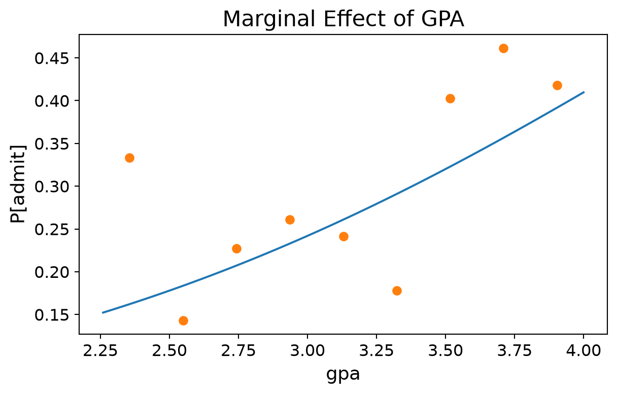
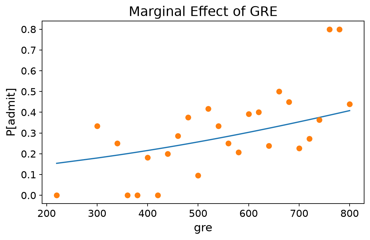
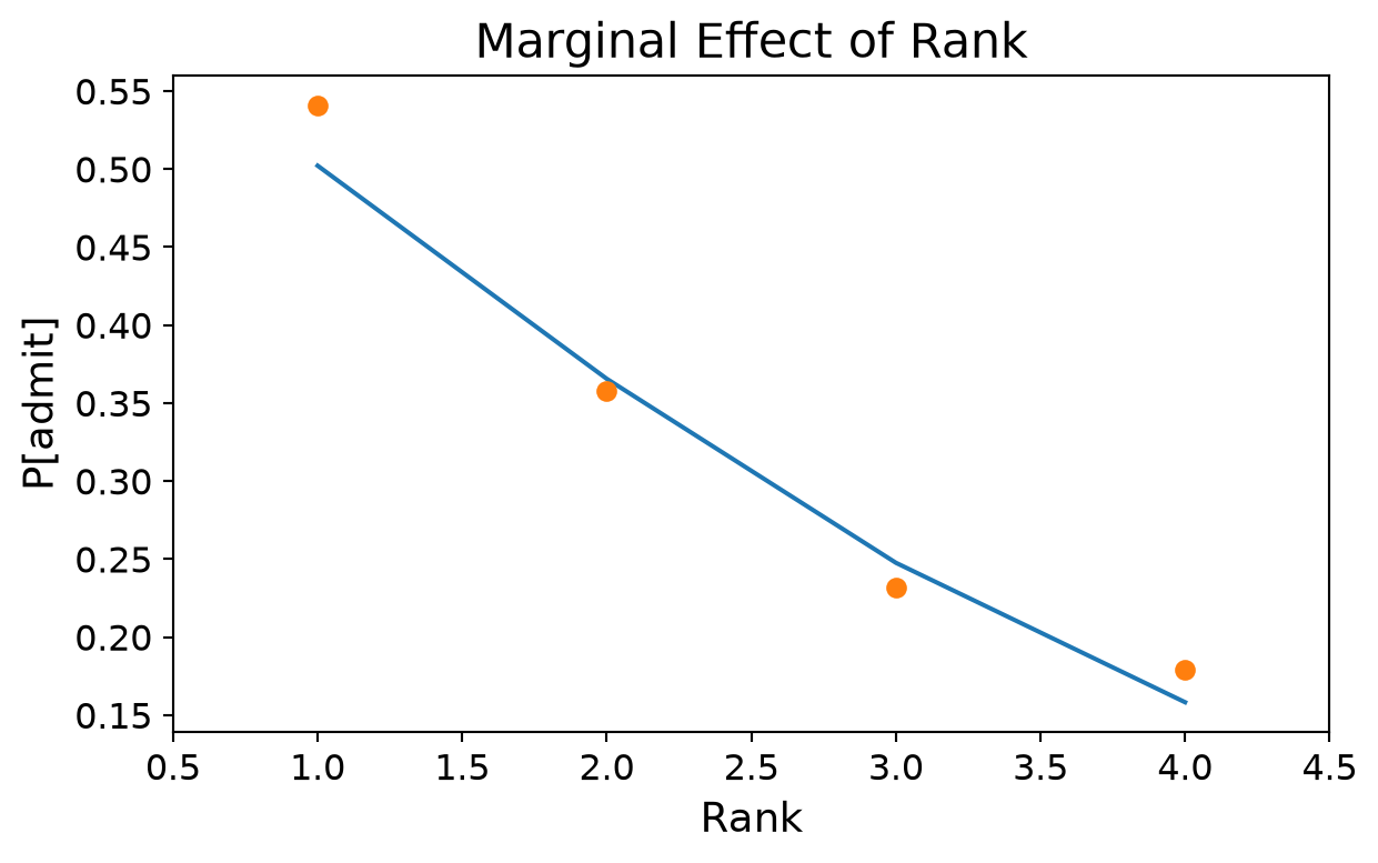
Let’s see how well the model fits the data.
We have three independent variables, so in each case we’ll use average values for the two that we aren’t evaluating.
GPA (GRE = 600, Rank = 2.5):
Code
gpa_grid = np.linspace(df.gpa.min(), df.gpa.max(), 50)prob = [result.predict([600, g, 2.5, 1.0]) for g in gpa_grid]bins = np.linspace(df.gpa.min(), df.gpa.max(), 10)groups = df.groupby(pd.cut(df.gpa, bins, include_lowest=True), observed=True)['admit'].mean()centers = [interval.mid for interval in groups.index]ax = plt.figure(figsize = (7, 4)).add_subplot()ax.plot(gpa_grid, prob)ax.plot(centers, groups, 'o')ax.tick_params(labelsize=12)ax.set_xlabel('gpa', fontsize =14)ax.set_ylabel('P[admit]', fontsize =14)ax.set_title('Marginal Effect of GPA', fontsize =16);
GRE Score (GPA = 3.4, Rank = 2.5):
Code
prob = [result.predict([b, 3.4, 2.5, 1.0]) for b insorted(df.gre.unique())]ax = plt.figure(figsize = (7, 4)).add_subplot()ax.plot(sorted(df.gre.unique()), prob)ax.plot(df.groupby('gre').mean()['admit'],'o')ax.tick_params(labelsize=12)ax.set_xlabel('gre', fontsize =14)ax.set_ylabel('P[admit]', fontsize =14)ax.set_title('Marginal Effect of GRE', fontsize =16);
Institution Rank (GRE = 600, GPA = 3.4):
Code
prob = [result.predict([600, 3.4, b, 1.0]) for b inrange(1,5)]ax = plt.figure(figsize = (7, 4)).add_subplot()ax.plot(range(1,5), prob)ax.plot(df.groupby('rank').mean()['admit'],'o')ax.tick_params(labelsize=12)ax.set_xlabel('Rank', fontsize =14)ax.set_xlim([0.5,4.5])ax.set_ylabel('P[admit]', fontsize =14)ax.set_title('Marginal Effect of Rank', fontsize =16);
Logistic Regression in Perspective
At the start of lecture we emphasized that logistic regression is concerned with estimating a probability model for discrete (0/1) data.
However, it may well be the case that we want to do something with the probability that amounts to classification.
For example, we may classify data items using a rule such as “Assign item \(\mathbf{x}_i\) to Class 1 if \(p(y_i{=}1 \mid \mathbf{x}_i) > 0.5\)”.
For this reason, logistic regression could be considered a classification method.
The decision boundary is still a hyperplane
The rule “\(p(y{=}1 \mid \mathbf{x}) > 0.5\)” is the rule “\(\boldsymbol{\beta}^T\mathbf{x} > 0\)”
the sigmoid is monotonic, so thresholding the probability is the same as thresholding the linear score.
The boundary \(\boldsymbol{\beta}^T\mathbf{x} = 0\) is a hyperplane – a line in two features – exactly as in the linear classifiers you have seen.
The nonlinearity lives in the confidence, not in the boundary.
Any other threshold \(t\) slides the hyperplane parallel to itself, to \(\boldsymbol{\beta}^T\mathbf{x} = \text{logit}(t)\).
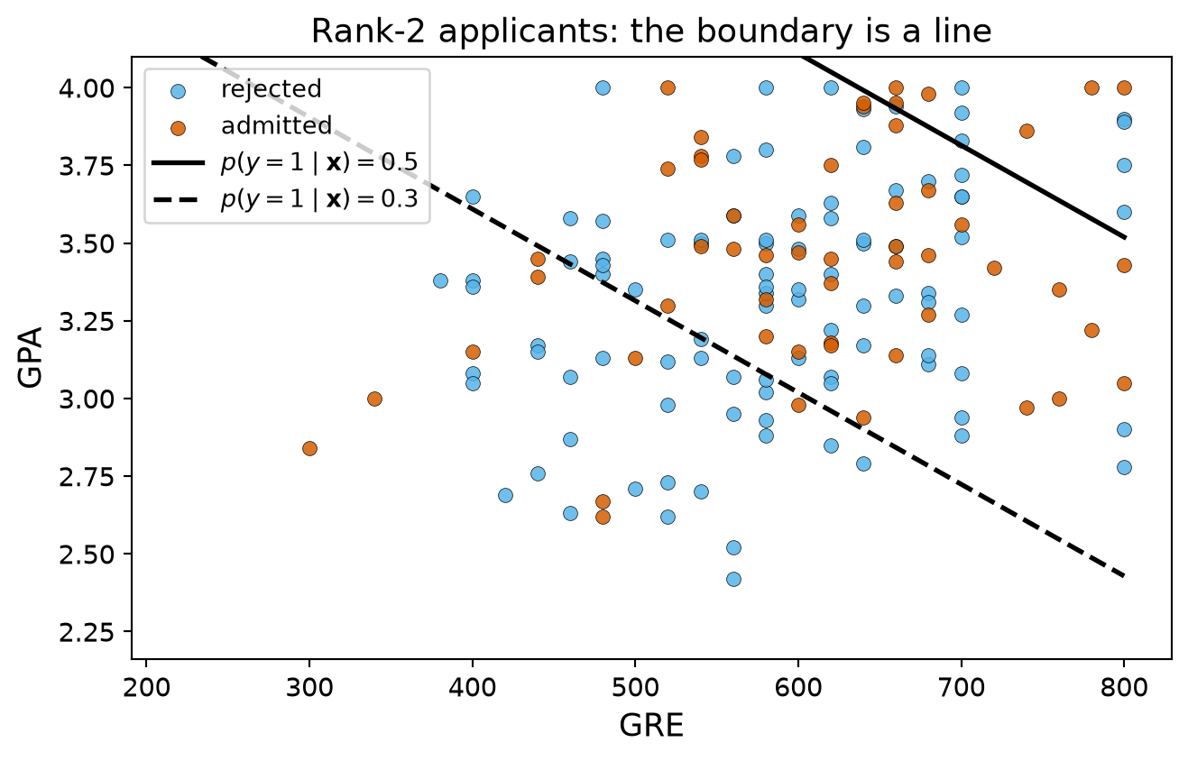
Rank-2 applicants, with the boundary \(\hat{\boldsymbol{\beta}}^T\mathbf{x} = \text{logit}(t)\) drawn for \(t = 0.5\) and \(t = 0.3\) (solved for GPA as a function of GRE):
Above the line the model says “admit”. At \(t = 0.5\) almost no rank-2 applicant qualifies; lowering the threshold to \(0.3\) slides the same line down into the cloud. Changing the threshold never bends the boundary.
Let’s use our logistic regression as a classifier.
We want to ask whether we can correctly predict whether a student gets admitted to graduate school.
avgPrec = np.mean([f[0] for f in PR])avgRec = np.mean([f[1] for f in PR])avgAcc = np.mean([f[2] for f in PR])print(f'Average Precision: {avgPrec:0.3f}, Average Recall: {avgRec:0.3f}, Average Accuracy: {avgAcc:0.3f}')
Average Precision: 0.612, Average Recall: 0.258, Average Accuracy: 0.712
Sometimes we would like a single value that describes the overall performance of the classifier.
For this, we take the harmonic mean of precision and recall, called F1 Score:
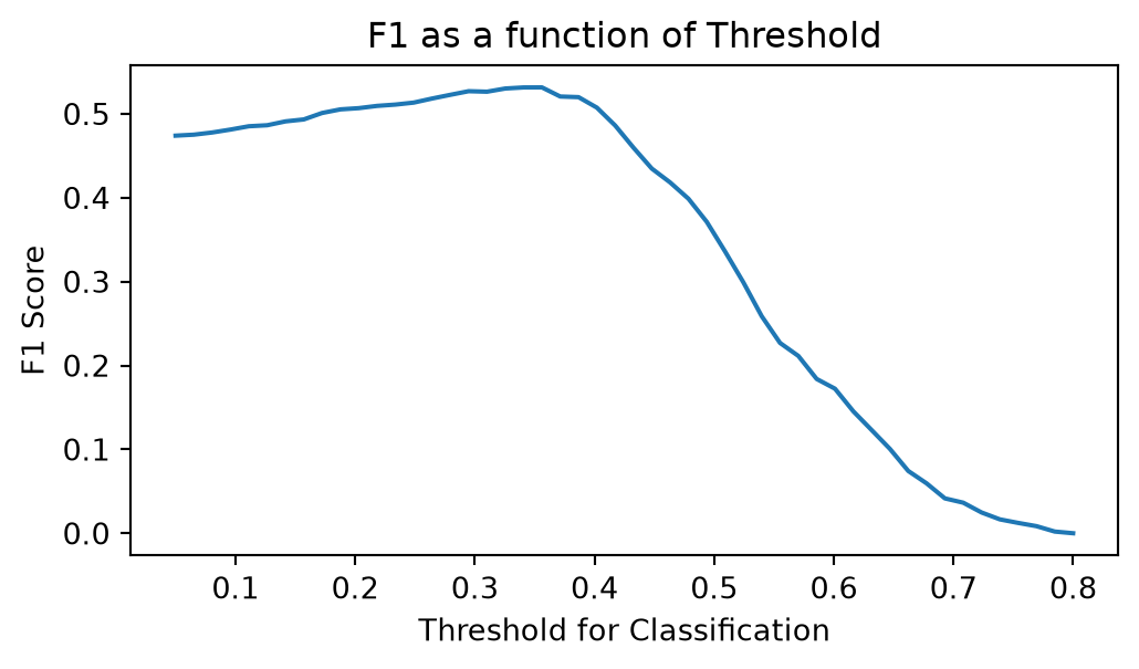
Using this, we can evaluate other settings for the threshold.
Code
def evalThresh(df, thresh): PR = []for i inrange(20): X_train, X_test, y_train, y_test = model_selection.train_test_split( df[train_cols], df['admit'], test_size=0.4, random_state=i) PR.append(evaluate(y_train, X_train, y_test, X_test, thresh)) avgPrec = np.mean([f[0] for f in PR]) avgRec = np.mean([f[1] for f in PR])# at high thresholds the model predicts no positives at all: F1 is 0, not 0/0 f1 =0.0if avgPrec + avgRec ==0else2* (avgPrec * avgRec) / (avgPrec + avgRec)return f1, avgPrec, avgRectvals = np.linspace(0.05, 0.8, 50)f1vals = [evalThresh(df, tval)[0] for tval in tvals]
Code
plt.figure(figsize=(6, 3))plt.plot(tvals,f1vals)plt.ylabel('F1 Score')plt.xlabel('Threshold for Classification')plt.title('F1 as a function of Threshold');
Based on this plot, we can say that the best classification threshold appears to be around 0.35 – well below 0.5 – where precision and recall are:
Compared with the 0.5 threshold we traded precision for recall: the model now says yes to most of the real admits, at the cost of more false alarms.
\(0.5\) is not a law of nature: it is where the model thinks the two classes are equally likely, which says nothing about what the two kinds of mistake cost.
If a false positive costs \(C_{FP}\) and a false negative costs \(C_{FN}\), saying “yes” is worth it exactly when \(p\,C_{FN} > (1-p)\,C_{FP}\), i.e. when
\[
p > t^* = \frac{C_{FP}}{C_{FP} + C_{FN}}.
\]
A miss that is four times as costly as a false alarm puts the threshold at \(t^* = 0.2\). Choosing \(t\) is a decision about costs, and F1 is just one cost-free way to summarize the trade-off.
The example here is based on http://blog.yhathq.com/posts/logistic-regression-and-python.html where you can find additional details.
ROC-AUC Curve
Two rates, both out of the true classes:
True positive rate (TPR, = recall): \(\text{TP}/(\text{TP}+\text{FN})\), the fraction of real admits we say yes to.
False positive rate (FPR): \(\text{FP}/(\text{FP}+\text{TN})\), the fraction of real rejects we wrongly say yes to.
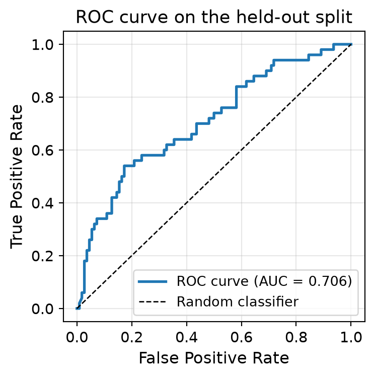
The ROC curve plots TPR against FPR, one point per threshold. The diagonal is a random classifier.
The AUC is the area under the ROC curve: a threshold-free summary of how well the model ranks admits above rejects.
Code
# Fit on a training split and score the held-out split -- a ROC curve on the# training data would flatter the model.X_train, X_test, y_train, y_test = model_selection.train_test_split( df[train_cols], df['admit'], test_size=0.4, random_state=1)roc_fit = sm.Logit(y_train, X_train).fit(disp=False)y_score = roc_fit.predict(X_test)fpr, tpr, thresholds = metrics.roc_curve(y_test, y_score)auc_score = metrics.roc_auc_score(y_test, y_score)fig, ax = plt.subplots(figsize=(4, 4))ax.plot(fpr, tpr, linewidth=2, label=f'ROC curve (AUC = {auc_score:.3f})')ax.plot([0, 1], [0, 1], 'k--', linewidth=1, label='Random classifier')ax.set_xlabel('False Positive Rate', fontsize=12)ax.set_ylabel('True Positive Rate', fontsize=12)ax.set_title('ROC curve on the held-out split', fontsize=13)ax.legend(loc='lower right', fontsize=10)ax.grid(True, alpha=0.3)ax.tick_params(labelsize=11)plt.tight_layout()plt.show()print(f"AUC Score: {auc_score:.4f}")
AUC Score: 0.7061
Recap: what you can now do
Write the logistic model – a linear function \(\boldsymbol{\beta}^T\mathbf{x}\) equal to the log-odds, inverted through the sigmoid \(\sigma\) – read \(\beta_j\) as a log-odds slope and \(e^{\beta_j}\) as an odds ratio, and explain why the decision boundary is still a hyperplane (the nonlinearity lives in the confidence).
Fit it by maximum likelihood: write the log-likelihood (minus the log-loss), use \(\sigma' = \sigma(1-\sigma)\) to get the gradient \(X^T(\mathbf{y}-\mathbf{p})\), take one gradient step by hand, and say why there is no closed form.
Evaluate a classifier beyond accuracy: accuracy has a floor set by prevalence; sweep the threshold, trade precision against recall and F1, and read ROC/AUC for what it does (ranking) and does not (choose a threshold) tell you.
Choose a threshold to ship: the cost-optimal threshold is \(C_{FP}/(C_{FP}+C_{FN})\) – in today’s activity you will sweep precision, recall and F1 on a held-out split of an imbalanced loan-default problem, read its ROC-AUC, and compare the cost-optimal threshold with \(0.5\) and with class_weight="balanced".
Next: Regularization (Lecture 11B)
Linear and logistic models can both overfit: with many or correlated features, \(\hat{\boldsymbol{\beta}}\) chases noise in the training set.
The fix is a penalty on the size of \(\boldsymbol{\beta}\): ridge and LASSO.
Lecture 11B develops it for linear regression and applies it to today’s logistic model.